Accounts Receivable Aging and Collections Priority Template for Excel
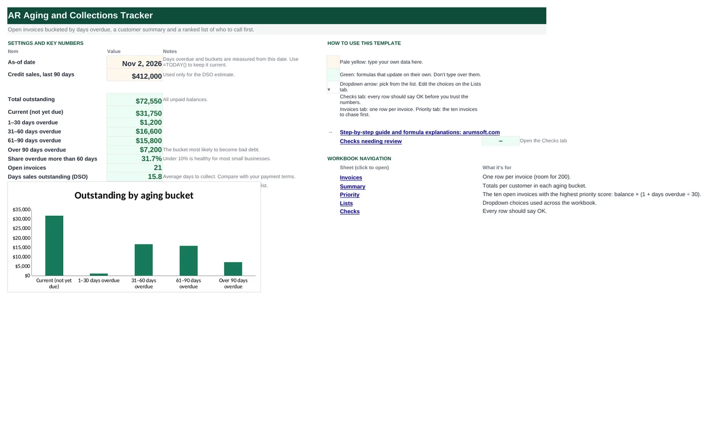
Type your open invoices once and the workbook does the aging: due dates from terms, days overdue from an as-of date, the standard buckets, totals per customer and a priority list that ranks invoices by balance and age so the first call of the day is the right one. Filled in with fictional customers.
- Sheets:
- 6
- Works with:
- Excel for Microsoft 365, Excel 2016 or later, Excel for Mac and Excel for the web
- Updated:
What you can do with it
- See how much is outstanding in each aging bucket, on one dashboard
- Get a per-customer summary with the oldest overdue invoice and a suggested next step
- Work a ranked top-10 list of invoices to chase first
- Estimate days sales outstanding (DSO) from your credit sales
What's inside
The workbook has 6 sheets. You only type on a few of them; the rest calculate.
| Sheet | What it's for | You enter | Calculated for you |
|---|---|---|---|
| Start Here | As-of date, totals by bucket, DSO, largest balance and a chart | As-of date, credit sales for the last 90 days | Total outstanding, five bucket totals, share over 60 days, open invoice count, DSO, largest customer balance |
| Invoices | One row per invoice (room for 200) | Invoice number, customer, invoice date, terms, amount, paid, notes | Due date, balance, days overdue, bucket, status, priority score |
| Summary | One row per customer (30) | Nothing: customer names come from Lists | Open invoices, amount per bucket, total, share overdue, oldest overdue, next step |
| Priority | The ten invoices to chase first | Nothing | Rank, invoice, customer, balance, days overdue, bucket, score, suggested action |
| Lists | Dropdown choices | Customer names, payment terms | Nothing |
| Checks | Six data checks | Nothing | OK or Review |
Before you start
- Export your open invoices from your invoicing system with invoice date, terms, amount and amount paid.
- Add every customer name to the Lists tab first so the Invoices dropdown and the Summary tab know them.
- Decide the as-of date. Most teams run aging on the last day of the month or every Monday.
Step-by-step guide
Set the as-of date
Start Here B6 is the date everything is measured from. Type a date, or enter =TODAY() to keep the aging current every time the file opens. B7 (credit sales in the last 90 days) is only used for the DSO estimate.
Add customers on the Lists tab
Column A of Lists is the customer dropdown and the row list on the Summary tab. One name per row, spelled exactly as you want it to appear.
Enter invoices
On the Invoices tab type the invoice number, pick the customer from the dropdown, enter the invoice date, pick the terms (days), and type the amount. When a payment arrives, type it in Paid; a fully paid invoice drops out of every total on its own.
Read the calculated columns
Due date is invoice date plus terms. Balance is amount minus paid. Days overdue counts from the due date to the as-of date (never negative). Bucket is Current, 1-30, 31-60, 61-90 or 90+; Status is Open or Paid; the Priority score weights balance by age.
Check the Summary tab
Each customer gets a row with their open invoice count, the amount in each bucket, the total, the share that is overdue, the oldest overdue invoice in days, and a suggested next step that escalates with age.
Work the Priority tab
Ten rows, ranked by priority score. Start at rank 1. The suggested action column says whether a reminder email, a call, a payment plan or a final notice fits the age of the invoice.
Review the Checks tab
The checks catch an invoice paid for more than its amount, missing customers, dates or terms, a customer on an invoice that is not on the Lists tab, and whether the five buckets add up to the total outstanding.
Formula map
Every formula in the workbook, grouped by the sheet and column it lives in. A column of copied formulas counts once; the range it covers is shown.
| Sheet | Cells | Functions | What it computes | Reads | Feeds |
|---|---|---|---|---|---|
| Invoices | E5 copied down to row 204 | IF | Due date | C5, D5 | Days overdue (column I) counts from this date. |
| Invoices | H5 copied down to row 204 | IF | Balance | F5, G5 | Used by every SUMIF on Start Here and Summary, and by the priority score. |
| Invoices | I5 copied down to row 204 | IF, OR, MAX | Days overdue | E5, H5 | The bucket in column J and the priority score in column L both read this. |
| Invoices | J5 copied down to row 204 | IF | Aging bucket | H5, I5 | Start Here sums balances per bucket by matching these words exactly, so the Summary and Start Here SUMIFs use the same spellings. |
| Invoices | L5 copied down to row 204 | IF, OR, ROW | Priority score | H5, I5 | The Priority tab uses LARGE on this column to pick the top ten and MATCH to find each row. |
| Start Here | B10 | SUMIF | Outstanding per bucket | — | B15 uses the 61-90 and 90+ cells to compute the share overdue more than 60 days; the Checks tab confirms the five buckets add up to B9. |
| Start Here | B17 | IF | Days sales outstanding | B7, B9 | Compare with your standard terms: DSO of 45 on net-30 terms means customers pay two weeks late on average. |
| Start Here | B18 | INDEX, MATCH, MAX | Largest customer balance | — | A quick pointer to the account that matters most. |
| Summary | B5 copied down to row 34 | IF, COUNTIFS | Open invoices per customer | — | Shown next to the bucket amounts. |
| Summary | C5 copied down to row 34 | IF, SUMIFS | Amount per bucket per customer | — | H5 totals the five buckets; I5 computes the overdue share. |
| Summary | J5 copied down to row 34 | IF, MAXIFS | Oldest overdue invoice (days) | — | K5 turns this number into a next step. |
| Summary | K5 copied down to row 34 | IF | Suggested next step | — | The Priority tab uses the same ladder per invoice. |
| Priority | G5 copied down to row 14 | IFERROR, LARGE | Nth highest priority score | — | B5 to F5 look up the invoice that owns this score. |
| Priority | B5 copied down to row 14 | IF, INDEX, MATCH | Invoice details for that score | — | This is the call list. |
| Checks | B6 | IF, SUMPRODUCT | No invoice overpaid | — | An overpayment usually means a typo in Paid. |
| Checks | B10 | IF, SUMPRODUCT, ISNA, MATCH | Every invoice customer is on the Lists tab | — | Fix by adding the name to Lists or correcting the spelling on the invoice. |
Every formula, explained
Each formula below is copied straight from the file, so what you read here is exactly what the cell contains. Click any cell in Excel to see it in the formula bar.
=IF(C5="", "", C5+D5)Invoice date plus the payment terms in days. Blank until an invoice date is typed.
Piece by piece
C5=""- No invoice date yet: show nothing.
C5+D5- Date plus days. Excel dates are day numbers, so adding 30 gives the date 30 days later.
With the sample data: C5 = Jun 17, 2026, D5 = 30 → E5 result Jul 17, 2026
How it is used: Days overdue (column I) counts from this date.
How to change it: For terms like "end of month plus 30", replace C5+D5 with EOMONTH(C5,0)+30.
Learn this: Text and Date Functions in Excel →=IF(F5="", "", F5-G5)Amount minus what has been paid. This is the number every total on the other tabs adds up.
Piece by piece
F5=""- No amount yet: show nothing.
F5-G5- Amount minus paid. A blank Paid cell counts as zero.
With the sample data: F5 = 4,800, G5 = 0 → H5 result 4,800
How it is used: Used by every SUMIF on Start Here and Summary, and by the priority score.
How to change it: Nothing to change.
Learn this: How to Write Basic Formulas in Excel →=IF(OR(F5="", H5<=0), "", MAX(0, 'Start Here'!$B$6-E5))Days between the due date and the as-of date, floored at zero so invoices that are not yet due show 0.
Piece by piece
OR(F5="", H5<=0)- Skip blank rows and paid invoices: show nothing.
'Start Here'!$B$6-E5- As-of date minus due date, in days. The as-of reference is absolute so it stays fixed when the formula is copied down.
MAX(0, …)- Negative results (not yet due) become 0.
With the sample data: E5 = Jul 17, 2026, H5 = 4,800 → I5 result 108
How it is used: The bucket in column J and the priority score in column L both read this.
How to change it: Nothing to change; edit the as-of date on Start Here.
Learn this: How to Use MIN and MAX in Excel →=IF(F5="", "", IF(H5<=0, "Paid",
IF(I5=0, "Current", IF(I5<=30, "1-30", IF(I5<=60, "31-60", IF(I5<=90, "61-90", "90+"))))))A chain of IF tests from the smallest age up. Order matters: because each test only runs when the previous one failed, "<=60" really means 31 to 60.
Piece by piece
F5=""- Blank row: show nothing.
H5<=0- Nothing owed: "Paid".
I5=0- Not yet due: "Current".
I5<=30, I5<=60, I5<=90- The 1-30, 31-60 and 61-90 buckets, tested in order.
"90+"- Everything older.
With the sample data: H5 = 4,800, I5 = 108 → J5 result 90+
How it is used: Start Here sums balances per bucket by matching these words exactly, so the Summary and Start Here SUMIFs use the same spellings.
How to change it: To change the bucket edges (say 45 and 90), change the numbers here and the labels on Start Here and Summary.
Learn this: Logic Formulas in Excel: IF with AND, OR and IFS →=IF(OR(F5="", H5<=0), 0, H5*(1+I5/30)+ROW()/1000000)Balance weighted by how late it is: each 30 days overdue adds 100% of the balance again. A tiny row-based tie-breaker makes every score unique so the Priority tab can look rows up without collisions.
Piece by piece
OR(F5="", H5<=0)- Blank or paid rows score 0 so they never rank.
H5*(1+I5/30)- Balance × (1 + months overdue).
ROW()/1000000- Adds a millionth of the row number: invisible in the ranking, but it guarantees no two scores are exactly equal.
With the sample data: H5 = 4,800, I5 = 108 → L5 result 22,080
How it is used: The Priority tab uses LARGE on this column to pick the top ten and MATCH to find each row.
How to change it: Change the 30 to 15 to weight age twice as heavily.
Learn this: How to Write Basic Formulas in Excel →=SUMIF(Invoices!$J$5:$J$204, "Current", Invoices!$H$5:$H$204)Adds the balances of invoices whose bucket word matches. B11 to B14 are the same formula with the other bucket names.
Piece by piece
Invoices!$J$5:$J$204- The bucket column: the range to test.
"Current"- The bucket to add up.
Invoices!$H$5:$H$204- The balance column: the range to sum.
With the sample data: B10 result 31,750
How it is used: B15 uses the 61-90 and 90+ cells to compute the share overdue more than 60 days; the Checks tab confirms the five buckets add up to B9.
How to change it: Nothing to change unless you rename the buckets.
Learn this: How to Use SUMIF and SUMIFS in Excel →=IF(B7=0, 0, B9/(B7/90))Outstanding receivables divided by average daily credit sales. The 90 matches the "last 90 days" input.
Piece by piece
B7=0- Guard against dividing by zero when no sales figure is entered.
B9/(B7/90)- Total outstanding ÷ (90-day credit sales ÷ 90 days).
With the sample data: B7 = 412,000, B9 = 72,550 → B17 result 15.85
How it is used: Compare with your standard terms: DSO of 45 on net-30 terms means customers pay two weeks late on average.
How to change it: If you enter a full year of credit sales instead, change 90 to 365.
Learn this: How to Write Basic Formulas in Excel →=INDEX(Summary!$A$5:$A$34,
MATCH(MAX(Summary!$H$5:$H$34),
Summary!$H$5:$H$34, 0))Finds the highest total on the Summary tab and returns the customer name in the same row.
Piece by piece
MAX(Summary!$H$5:$H$34)- The biggest total outstanding.
MATCH(…, Summary!$H$5:$H$34, 0)- Which row holds it.
INDEX(Summary!$A$5:$A$34, …)- The customer name in that row.
With the sample data: B18 result Harbor Logistics
How it is used: A quick pointer to the account that matters most.
How to change it: Nothing to change.
Learn this: How to Use INDEX and MATCH in Excel →=IF(A5="", "", COUNTIFS(Invoices!$B$5:$B$204,
A5, Invoices!$K$5:$K$204,
"Open"))Counts invoices that belong to the customer and are still open.
Piece by piece
$A5=""- No customer in this row: show nothing. The column is anchored with $ so the same test works in every column of the row.
Invoices!$B$5:$B$204, A5- Customer column equals this row's customer.
Invoices!$K$5:$K$204, "Open"- Status column equals Open.
With the sample data: B5 result 1
How it is used: Shown next to the bucket amounts.
How to change it: Nothing to change.
Learn this: How to Use COUNTIF and COUNTIFS in Excel →=IF($A5="", "", SUMIFS(Invoices!$H$5:$H$204,
Invoices!$B$5:$B$204, $A5,
Invoices!$J$5:$J$204, "Current"))Two conditions: the customer matches and the bucket matches. Columns D to G repeat it with the other bucket names.
Piece by piece
Invoices!$H$5:$H$204- Balances to sum.
Invoices!$B$5:$B$204, $A5- Customer condition. $A5 keeps the customer column fixed when copying across.
Invoices!$J$5:$J$204, "Current"- Bucket condition.
With the sample data: C5 result 3,150
How it is used: H5 totals the five buckets; I5 computes the overdue share.
How to change it: Nothing to change unless you rename the buckets.
Learn this: How to Use SUMIF and SUMIFS in Excel →=IF(A5="", "", MAXIFS(Invoices!$I$5:$I$204,
Invoices!$B$5:$B$204, A5,
Invoices!$K$5:$K$204, "Open"))The largest days-overdue value among the customer's open invoices. MAXIFS is available in Excel 2019 and Microsoft 365.
Piece by piece
Invoices!$I$5:$I$204- Days overdue: the values to take the maximum of.
Invoices!$B$5:$B$204, A5- Customer condition.
Invoices!$K$5:$K$204, "Open"- Only open invoices.
With the sample data: J5 result 0
How it is used: K5 turns this number into a next step.
How to change it: On Excel 2016, replace with =MAX(IF((Invoices!$B$5:$B$204=A5)*(Invoices!$K$5:$K$204="Open"),Invoices!$I$5:$I$204)) entered with Ctrl+Shift+Enter.
Learn this: How to Use MIN and MAX in Excel →=IF(A5="", "", IF(H5=0, "Nothing open",
IF(J5>90, "Final notice or collections", IF(J5>60, "Call and payment plan", IF(J5>30, "Call", "Reminder email")))))Escalates the collection action with the age of the oldest overdue invoice.
Piece by piece
H5=0- Nothing outstanding: "Nothing open".
J5>90, J5>60, J5>30- Thresholds for final notice, call and payment plan, call.
"Reminder email"- Everything 30 days or less.
With the sample data: K5 result Reminder email
How it is used: The Priority tab uses the same ladder per invoice.
How to change it: Edit the words to match your own collections policy.
Learn this: Logic Formulas in Excel: IF with AND, OR and IFS →=IFERROR(LARGE(Invoices!$L$5:$L$204, A5), 0)LARGE returns the k-th largest value, where k is the rank in column A. Blank-safe: if there are fewer open invoices than ranks, IFERROR shows 0 and the row stays empty.
Piece by piece
Invoices!$L$5:$L$204- All priority scores.
A5- The rank: 1 for the highest, 2 for the next, and so on.
IFERROR(…, 0)- When there is no k-th invoice.
With the sample data: G5 result 35,280
How it is used: B5 to F5 look up the invoice that owns this score.
How to change it: To show 20 rows, copy row 14 down and type ranks 11–20.
Learn this: How to Use MIN and MAX in Excel →=IF(G5=0, "", INDEX(Invoices!$A$5:$A$204,
MATCH(G5, Invoices!$L$5:$L$204, 0)))Finds the row whose score equals the rank's score and returns the invoice number; columns C to F return customer, balance, days overdue and bucket from the same row.
Piece by piece
G5=0- No invoice at this rank: show nothing.
MATCH(G5, Invoices!$L$5:$L$204, 0)- Row position of that score. Scores are unique thanks to the tie-breaker, so the match is always the right invoice.
INDEX(Invoices!$A$5:$A$204, …)- The invoice number in that row.
With the sample data: B5 result INV-1043
How it is used: This is the call list.
How to change it: Nothing to change.
Learn this: How to Use INDEX and MATCH in Excel →=IF(SUMPRODUCT((Invoices!$G$5:$G$204>Invoices!$F$5:$F$204)*1)=0,
"OK", "Review")Counts rows where Paid is greater than Amount by multiplying a TRUE/FALSE array by 1 and adding it up.
Piece by piece
Invoices!$G$5:$G$204>Invoices!$F$5:$F$204- An array of TRUE/FALSE, one per row.
*1- Turns TRUE into 1 and FALSE into 0.
SUMPRODUCT(…)- Adds them: the number of overpaid rows.
With the sample data: B6 result OK
How it is used: An overpayment usually means a typo in Paid.
How to change it: Nothing to change.
Learn this: How to Use SUMIF and SUMIFS in Excel →=IF(SUMPRODUCT((Invoices!$B$5:$B$204<>"")*ISNA(MATCH(Invoices!$B$5:$B$204, Lists!$A$5:$A$34, 0)))=0,
"OK", "Review")Flags customers typed on the Invoices tab that do not exist on Lists, which would make them vanish from the Summary.
Piece by piece
Invoices!$B$5:$B$204<>""- Only rows with a customer.
ISNA(MATCH(…, Lists!$A$5:$A$34, 0))- TRUE when the name is not found on Lists.
SUMPRODUCT(…)- Counts the problem rows.
With the sample data: B10 result OK
How it is used: Fix by adding the name to Lists or correcting the spelling on the invoice.
How to change it: Nothing to change.
Learn this: How to Use INDEX and MATCH in Excel →Tips and limits
- Capacity: 200 invoices and 30 customers. To extend, press Ctrl+H, set Within to Workbook and Look in to Formulas, and replace $204 with $1004 (and $34 with a larger row for customers).
- Enter partial payments in the Paid column as they arrive; the balance and bucket update and the invoice leaves the list only when fully paid.
- Type =TODAY() in the as-of date to keep the aging live, but type a fixed date before saving a month-end copy so the snapshot does not change later.
- The DSO here is a simple estimate; accounting systems compute it over a trailing period with the same formula.
Learn the skills behind this template
Was this guide helpful? Spot a mistake? Send feedback · admin@arumsoft.com