SaaS Unit Economics Calculator for Excel: CAC, LTV and Payback
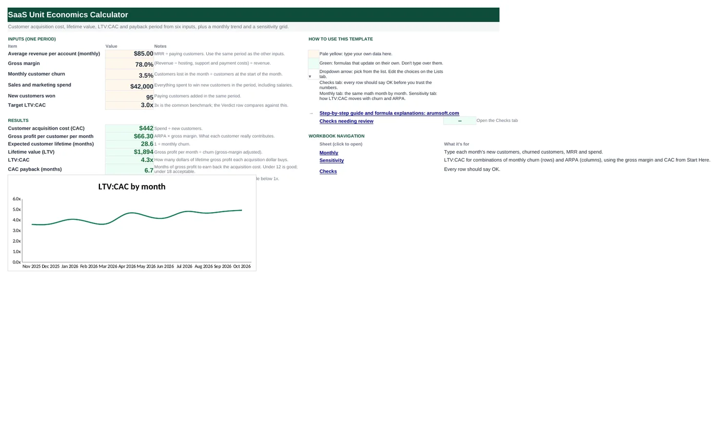
Six inputs on one sheet give you the four numbers investors ask about: CAC, LTV, LTV:CAC and payback months. A monthly tab repeats the math for the last 12 months so you can see the trend, and a sensitivity grid shows how LTV:CAC moves when churn or pricing changes. Filled in with sample figures for a fictional product.
- Sheets:
- 4
- Works with:
- Excel for Microsoft 365, Excel 2016 or later, Excel for Mac and Excel for the web
- Updated:
What you can do with it
- Compute CAC, LTV, LTV:CAC and CAC payback from six inputs
- Track the same metrics month by month for a year
- See which churn and ARPA combinations clear your target ratio
- Get a plain-language verdict: Healthy, Marginal or Unprofitable
What's inside
The workbook has 4 sheets. You only type on a few of them; the rest calculate.
| Sheet | What it's for | You enter | Calculated for you |
|---|---|---|---|
| Start Here | Inputs, results, verdict and the monthly LTV:CAC chart | ARPA, gross margin, monthly churn, sales and marketing spend, new customers, target ratio | CAC, gross profit per customer, lifetime, LTV, LTV:CAC, payback, verdict |
| Monthly | 12 months of the same math | Starting customers, and for each month: new, churned, MRR, spend | Ending customers, ARPA, churn rate, CAC, LTV, LTV:CAC, payback, net new, averages |
| Sensitivity | LTV:CAC grid: churn down the side, ARPA across the top | The churn and ARPA values on the edges | Every cell of the grid, colored against the target |
| Checks | Five input checks | Nothing | OK or Review |
Before you start
- Pick one period (a month or a quarter) and take every input from that same period.
- Gross margin should subtract hosting, third-party fees, support and onboarding costs that scale with customers; not sales or R&D.
- Churn is customers lost ÷ customers at the start of the period. Enter 2.5% as 0.025 or type 2.5% directly.
Step-by-step guide
Enter the six inputs
Start Here B6 to B11: average revenue per account per month, gross margin, monthly churn, sales and marketing spend for the period, the number of new customers won in that period, and your target LTV:CAC (3x is the usual benchmark).
Read the results block
CAC is spend ÷ new customers. Gross profit per customer is ARPA × margin. Lifetime is 1 ÷ churn. LTV is gross profit per month ÷ churn. LTV:CAC is the ratio. Payback is CAC ÷ monthly gross profit. The verdict compares LTV:CAC with your target.
Fill in the Monthly tab
Type the customers you had before month 1 in B5, then for each month the new customers, churned customers, MRR and spend. Ending customers, ARPA, churn rate, CAC, LTV, LTV:CAC and payback calculate per month, with 12-month averages at the bottom and a chart on Start Here.
Explore the Sensitivity tab
The grid uses the CAC and gross margin from Start Here and shows LTV:CAC for eight churn rates against eight ARPA values. Green cells clear the target; red cells are below 1x. Edit the yellow edge values to test your own scenarios.
Check the Checks tab
Catches a churn rate entered as a whole number (2.5 instead of 2.5%), a gross margin over 100%, missing spend or customer counts, and monthly rows where churn exceeds the starting customer count.
Formula map
Every formula in the workbook, grouped by the sheet and column it lives in. A column of copied formulas counts once; the range it covers is shown.
| Sheet | Cells | Functions | What it computes | Reads | Feeds |
|---|---|---|---|---|---|
| Start Here | B14 copied down to row 19 | IF | Customer acquisition cost | B9, B10 | Used by LTV:CAC (B18), payback (B19), the Monthly tab average and the whole Sensitivity grid. |
| Start Here | B15 | arithmetic | Gross profit per customer per month | B6, B7 | The numerator of LTV and the denominator of payback. |
| Start Here | B17 | IF | Lifetime value | B15, B8 | Compared with CAC in B18. |
| Start Here | B18 | IF | LTV:CAC ratio | B17, B14 | The verdict in B20 and the Monthly tab's conditional formatting both compare against the target in B11. |
| Start Here | B19 copied down to row 19 | IF | CAC payback in months | B14, B15 | Under 12 months is strong for SMB SaaS; 18 to 24 is typical for enterprise. |
| Start Here | B20 | IF | Verdict | B18, B11 | A quick read for a slide or a board update. |
| Monthly | E6 copied down to row 17 | arithmetic | Ending customers | B6, C6, D6 | ARPA (H) divides MRR by this count. |
| Monthly | I6 copied down to row 17 | IF | Monthly churn rate | D6, B6 | LTV in column K divides by this. |
| Monthly | K6 copied down to row 17 | IF | LTV per month | H6, I6 | L6 divides this by the month's CAC. |
| Monthly | C18 copied across to column N | AVERAGE | 12-month averages | — | Compare with the single-period inputs on Start Here to see whether one month is an outlier. |
| Sensitivity | B5 copied down to row 12 | IF, OR | LTV:CAC for one churn/ARPA pair | — | Conditional formatting colors the cell green at or above the target and red below 1x. |
| Checks | B6 | IF, AND | Churn entered as a monthly rate | — | A Review here means every result is wrong by a factor of 100. |
Every formula, explained
Each formula below is copied straight from the file, so what you read here is exactly what the cell contains. Click any cell in Excel to see it in the formula bar.
=IF(B10=0, 0, B9/B10)Everything spent to win customers divided by the customers won. The IF guards against a blank or zero customer count.
Piece by piece
B10=0- No new customers: show 0 instead of a #DIV/0! error.
B9/B10- Sales and marketing spend ÷ new customers.
With the sample data: B9 = 42,000, B10 = 95 → B14 result 442.11
How it is used: Used by LTV:CAC (B18), payback (B19), the Monthly tab average and the whole Sensitivity grid.
How to change it: If you track blended and paid CAC separately, add a second spend cell and a second CAC row.
Learn this: How to Write Basic Formulas in Excel →=B6*B7ARPA multiplied by gross margin: what a customer actually contributes each month after the costs of serving them.
Piece by piece
B6- Average revenue per account, monthly.
B7- Gross margin as a fraction (0.78 = 78%).
With the sample data: B6 = 85, B7 = 78.0% → B15 result 66.3
How it is used: The numerator of LTV and the denominator of payback.
How to change it: Nothing to change.
Learn this: How to Write Basic Formulas in Excel →=IF(B8=0, 0, B15/B8)Monthly gross profit divided by monthly churn. Dividing by churn is the same as multiplying by the expected lifetime in months (B16 = 1 ÷ churn).
Piece by piece
B8=0- Zero churn would mean infinite lifetime: show 0 rather than an error.
B15/B8- Gross profit per month ÷ churn rate.
With the sample data: B15 = 66.3, B8 = 3.5% → B17 result 1,894.29
How it is used: Compared with CAC in B18.
How to change it: For a more conservative LTV, cap the lifetime: use B15*MIN(1/B8, 36) for a 36-month ceiling.
Learn this: How to Write Basic Formulas in Excel →=IF(B14=0, 0, B17/B14)Lifetime value divided by acquisition cost. Formatted as 0.0"x" so 4.3 displays as 4.3x.
Piece by piece
B14=0- No CAC yet: show 0.
B17/B14- LTV ÷ CAC.
With the sample data: B17 = 1,894.29, B14 = 442.11 → B18 result 4.28
How it is used: The verdict in B20 and the Monthly tab's conditional formatting both compare against the target in B11.
How to change it: Nothing to change.
Learn this: Number and Date Formats in Excel →=IF(B15=0, 0, B14/B15)How many months of gross profit it takes to earn back the acquisition cost.
Piece by piece
B15=0- No gross profit: show 0.
B14/B15- CAC ÷ gross profit per customer per month.
With the sample data: B14 = 442.11, B15 = 66.3 → B19 result 6.67
How it is used: Under 12 months is strong for SMB SaaS; 18 to 24 is typical for enterprise.
How to change it: Nothing to change.
Learn this: How to Write Basic Formulas in Excel →=IF(B18>=B11, "Healthy", IF(B18>=1,
"Marginal", "Unprofitable"))A nested IF that turns the ratio into a word.
Piece by piece
B18>=B11- At or above the target: "Healthy".
B18>=1- Between 1x and the target: "Marginal".
"Unprofitable"- Below 1x: each customer costs more than it will ever return.
With the sample data: B18 = 4.28, B11 = 3 → B20 result Healthy
How it is used: A quick read for a slide or a board update.
How to change it: Change the words or the thresholds to match your own policy.
Learn this: How to Use the IF Function in Excel →=B6+C6-D6Starting customers plus new minus churned. The next month's starting count (column B) links to this cell, so the chain rolls forward automatically.
Piece by piece
B6- Customers at the start of the month (month 1 links to B5; later months link to the previous ending count).
C6- New customers.
D6- Churned customers.
With the sample data: B6 = 420, C6 = 38, D6 = 9 → E6 result 449
How it is used: ARPA (H) divides MRR by this count.
How to change it: Nothing to change.
Learn this: How to Write Basic Formulas in Excel →=IF(B6=0, 0, D6/B6)Churned customers divided by the customers you started the month with.
Piece by piece
B6=0- No customers at the start: show 0.
D6/B6- Churned ÷ starting.
With the sample data: D6 = 9, B6 = 420 → I6 result 2.1%
How it is used: LTV in column K divides by this.
How to change it: For revenue churn instead of logo churn, divide lost MRR by starting MRR.
Learn this: How to Write Basic Formulas in Excel →=IF(I6=0, 0, H6*'Start Here'!$B$7/I6)The same LTV formula as Start Here, using that month's ARPA and churn and the gross margin from Start Here B7 (absolute reference, because it is one assumption shared by every row).
Piece by piece
I6=0- No churn that month: show 0 rather than an infinite LTV.
H6*'Start Here'!$B$7- ARPA × gross margin = gross profit per customer.
/I6- ÷ churn rate.
With the sample data: H6 = 80.4, I6 = 2.1% → K6 result 2,926.59
How it is used: L6 divides this by the month's CAC.
How to change it: If gross margin changes month to month, add a column for it and replace the Start Here reference.
Learn this: Relative, Absolute and Mixed References in Excel →=AVERAGE(C6:C17)Plain averages of the monthly values. Row 18 repeats this for every calculated column.
Piece by piece
C6:C17- The twelve monthly values.
With the sample data: C18 result 59.58
How it is used: Compare with the single-period inputs on Start Here to see whether one month is an outlier.
How to change it: Nothing to change.
Learn this: How to Use the AVERAGE Function in Excel →=IF(OR($A5=0, 'Start Here'!$B$14=0),
0, (B$4*'Start Here'!$B$7/$A5)/'Start Here'!$B$14)The LTV formula with the ARPA taken from the column header and the churn from the row header, divided by the CAC on Start Here. The mixed references are what make one formula fill the whole grid.
Piece by piece
B$4- ARPA from the header row. The $ before the row number keeps it on row 4 when copied down.
$A5- Churn from the first column. The $ before the column letter keeps it in column A when copied across.
'Start Here'!$B$7- Gross margin, fully absolute.
'Start Here'!$B$14- CAC, fully absolute.
With the sample data: B5 result 9.7
How it is used: Conditional formatting colors the cell green at or above the target and red below 1x.
How to change it: Replace the edge values with your own ranges; the formulas do not need to change.
Learn this: Relative, Absolute and Mixed References in Excel →=IF(AND('Start Here'!$B$8>0,
'Start Here'!$B$8<0.5), "OK",
"Review")Catches the most common input mistake: typing 2.5 instead of 2.5%, which would make the lifetime 0.4 months.
Piece by piece
'Start Here'!$B$8>0- Churn must be positive.
'Start Here'!$B$8<0.5- A monthly churn above 50% is almost certainly a units error.
AND(…)- Both must be true for "OK".
With the sample data: B6 result OK
How it is used: A Review here means every result is wrong by a factor of 100.
How to change it: Nothing to change.
Learn this: How to Use AND and OR in Excel →Tips and limits
- LTV here is gross-margin adjusted and undiscounted. Investors sometimes also ask for a 3-year or 5-year capped LTV; the change tip on the LTV formula shows how.
- Use the same period for all six inputs. Mixing a quarter of spend with a month of new customers is the second most common error after the churn units.
- For a cohort-based view of retention rather than a single churn rate, use the Cohort Retention Matrix template on this site.
- Blended CAC (all spend ÷ all new customers) flatters paid channels when many customers arrive organically; split them if you can.
Learn the skills behind this template
Was this guide helpful? Spot a mistake? Send feedback · admin@arumsoft.com