13-Week Cash Flow Forecast Template for Excel
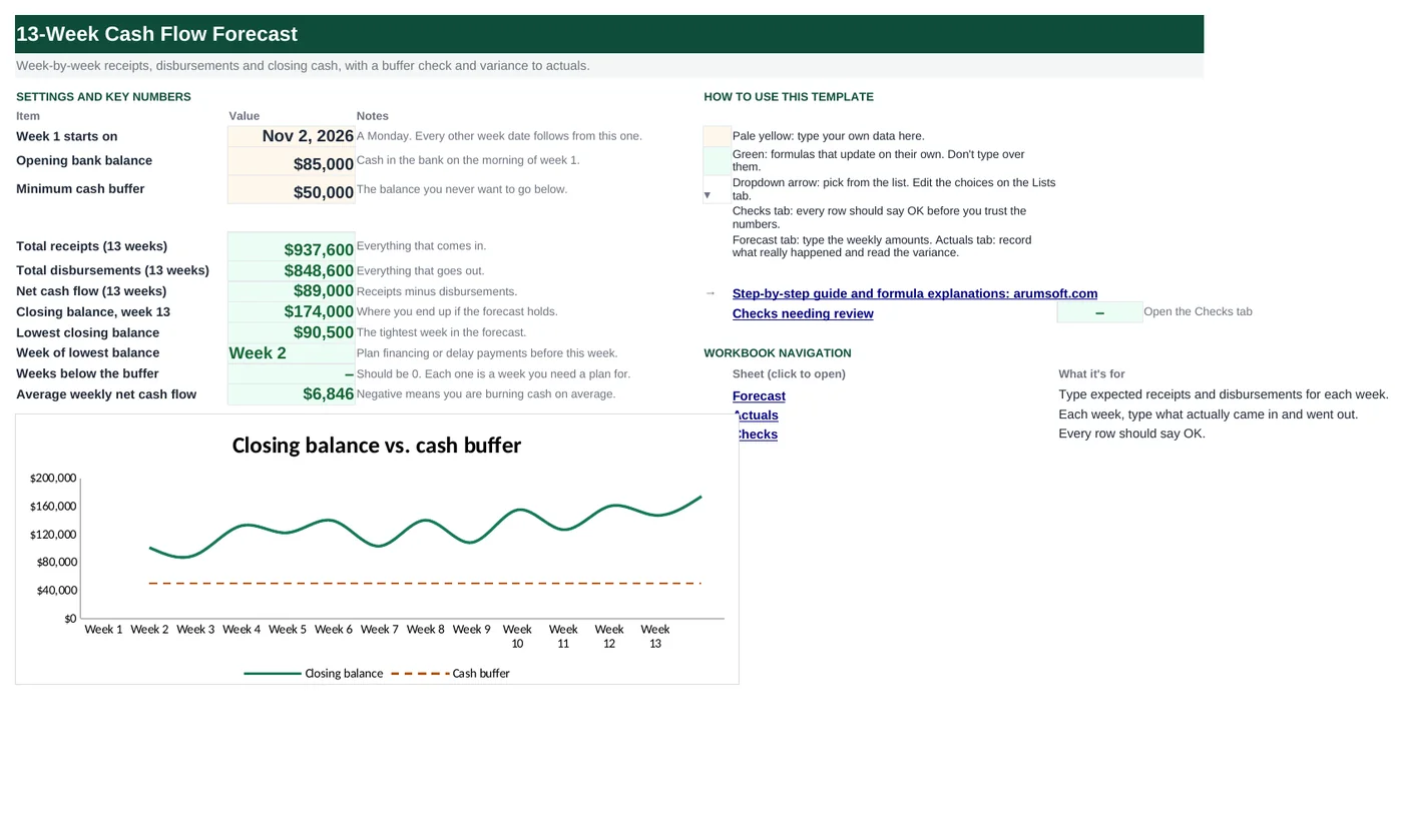
The weekly liquidity model finance teams use when cash is tight: type what you expect to collect and pay each week for 13 weeks, and the workbook chains the balances, flags any week that drops below your cash buffer, and compares the plan with what actually happened. Filled in for a fictional manufacturer so you can see the shape before you replace the numbers.
- Sheets:
- 4
- Works with:
- Excel for Microsoft 365, Excel 2016 or later, Excel for Mac and Excel for the web
- Updated:
What you can do with it
- See the closing cash balance for each of the next 13 weeks
- Find the lowest week and how far it sits above your buffer
- Record actuals each week and see the variance against the forecast
- Roll the forecast forward by changing one date
What's inside
The workbook has 4 sheets. You only type on a few of them; the rest calculate.
| Sheet | What it's for | You enter | Calculated for you |
|---|---|---|---|
| Start Here | Settings and key numbers, plus the closing-balance chart | Week 1 start date, opening bank balance, minimum cash buffer | Totals, net cash flow, week-13 closing balance, lowest week, weeks below buffer |
| Forecast | The 13-week grid: receipts, disbursements, net cash flow and closing balance | Line names and the weekly amounts | Week dates, opening balances, totals, net cash flow, closing balance, headroom, status |
| Actuals | What really happened, week by week | Actual receipts, disbursements and closing balance | Forecast figures pulled across, variances, totals to date |
| Checks | Six sanity checks | Nothing | OK or Review for each check |
Before you start
- Decide which bank accounts the forecast covers and use their combined balance as the opening balance.
- Pick a Monday for week 1. All other dates follow from it.
- Gather expected collections by week (open invoices and their due dates), the payroll calendar, rent and loan dates, and any tax deadlines in the next quarter.
Step-by-step guide
Set the three inputs on Start Here
Type the Monday that starts week 1 in B6, the bank balance that morning in B7, and the minimum balance you want to keep in B8. The buffer is what the Status row on the Forecast tab checks against.
Type weekly receipts on the Forecast tab
Rows 9–14 are cash coming in. Keep collections from receivables separate from cash sales so you can see which one is slipping. Customer deposits and other income have their own rows; two rows are spare.
Type weekly disbursements
Rows 18–27 are cash going out. Put payroll in the weeks it is actually paid (every other week in the sample), rent and loan payments in the weeks they leave the account, and taxes in the week they are due. The 13-week total in column P is a quick way to spot a line you forgot.
Read the closing balance and status rows
Row 31 is the balance at the end of each week; row 33 is how far above the buffer you are; row 34 says Below buffer in red for any week that dips under it. The chart on Start Here shows the same thing as a line against a dashed buffer line.
Fix the tight weeks
If a week shows Below buffer, the usual levers are: pull a collection forward (call the customer), push a supplier payment a week, or draw on a credit line. Change the number in the forecast grid and watch row 31 update.
Record actuals every week
On the Actuals tab, type the real receipts, disbursements and closing balance for the week that just ended. The variance columns show where the forecast was wrong; a pattern of over-forecasting collections is the most common finding.
Roll it forward
Each week, change the date in Start Here B6 to the next Monday, update B7 with the real balance, delete week 1 amounts and shift the rest left (or re-type them), and add week 13. Many teams keep a copy per week so the history survives.
Check the Checks tab
Every row should say OK. The checks catch a start date that is not a Monday, a missing opening balance, a week below the buffer, amounts on lines without a name, and actuals entered out of order.
Formula map
Every formula in the workbook, grouped by the sheet and column it lives in. A column of copied formulas counts once; the range it covers is shown.
| Sheet | Cells | Functions | What it computes | Reads | Feeds |
|---|---|---|---|---|---|
| Forecast | D5 copied across to column O | arithmetic | Week dates | C5 | Row 5 labels every column, and the Actuals tab looks these dates up by week number. |
| Forecast | D6 copied across to column O | arithmetic | Opening balance chain | C31 | Row 31 (closing balance) depends on this row, which depends on the previous closing balance: that chain is the whole model. |
| Forecast | C15 copied across to column P | SUM | Total receipts | C9, C10, C11, C12 | Net cash flow (row 30) subtracts total disbursements from this. |
| Forecast | C30 copied across to column P | arithmetic | Net cash flow | C15, C28 | Added to the opening balance in row 31. Start Here B17 averages this row. |
| Forecast | C31 copied across to column O | arithmetic | Closing balance | C6, C30 | Feeds the next week's opening balance, the headroom row, the status row, the chart and the Start Here metrics. |
| Forecast | C34 copied across to column O | IF | Below-buffer status | C31, C32 | Start Here B16 counts the weeks that fail this test (it uses the balances directly, with COUNTIF). |
| Start Here | B14 | MIN | Lowest closing balance | — | B15 finds which week it belongs to. |
| Start Here | B15 | INDEX, MATCH | Week of the lowest balance | B14 | Read it with B14: the week to prepare for. |
| Start Here | B16 | COUNTIF | Weeks below the buffer | B8 | The Checks tab expects this to be 0. |
| Actuals | C5 copied down to row 17 | INDEX | Forecast figures pulled across by week number | A5 | The variance in column E compares this with the actual you type in column D. |
| Actuals | E5 copied down to row 17 | IF | Receipts variance | C5, D5 | Row 19 totals the variances for the weeks that have actuals. |
| Actuals | C19 copied across to column F | SUMIF | Forecast total for weeks with actuals only | — | E19 compares it with the sum of actuals. |
| Checks | B5 | IF, WEEKDAY | Start date is a Monday | — | A forecast that starts mid-week makes payroll and rent land in the wrong columns. |
| Checks | B10 | IF, COUNT, IFERROR, MATCH, TRUE, INDEX | Actuals entered without gaps | — | A gap usually means a week was skipped. |
Every formula, explained
Each formula below is copied straight from the file, so what you read here is exactly what the cell contains. Click any cell in Excel to see it in the formula bar.
=C5+7Every week date is the previous week plus seven days, so changing the single date on Start Here moves the whole forecast.
Piece by piece
C5- The week-1 date, linked from Start Here B6.
+7- Seven days later. Excel stores dates as day numbers, so adding 7 adds a week.
With the sample data: C5 = Nov 2, 2026 → D5 result Nov 9, 2026
How it is used: Row 5 labels every column, and the Actuals tab looks these dates up by week number.
How to change it: For a fortnightly forecast change +7 to +14 and rename the headers.
Learn this: Text and Date Functions in Excel →=C31Each week opens with the balance the previous week closed with. Week 1 is the only exception: it links to the opening bank balance on Start Here.
Piece by piece
C31- The previous column's closing balance (row 31). The reference is relative, so when the formula is copied across, each week points at the column to its left.
With the sample data: C31 = 101,000 → D6 result 101,000
How it is used: Row 31 (closing balance) depends on this row, which depends on the previous closing balance: that chain is the whole model.
How to change it: Nothing to change. If you insert a week column, copy this formula into it so the chain stays unbroken.
Learn this: How to Write Basic Formulas in Excel →=SUM(C9:C14)Adds the six receipt lines for one week. The same formula sits under the disbursement lines (row 28, summing rows 18–27) and in column P for the 13-week totals.
Piece by piece
C9:C14- The receipt rows for this week. Blank cells count as zero, so spare rows do no harm.
With the sample data: C9 = 52,000, C10 = 9,000, C11 = 0, C12 = 0 → C15 result 61,000
How it is used: Net cash flow (row 30) subtracts total disbursements from this.
How to change it: If you add receipt rows below row 14, extend the range (for example C9:C16) in every column of row 15.
Learn this: How to Use the SUM Function in Excel →=C15-C28Receipts minus disbursements for the week. Negative means the week burned cash.
Piece by piece
C15- Total receipts for the week.
C28- Total disbursements for the week.
With the sample data: C15 = 61,000, C28 = 45,000 → C30 result 16,000
How it is used: Added to the opening balance in row 31. Start Here B17 averages this row.
How to change it: Nothing to change.
Learn this: How to Write Basic Formulas in Excel →=C6+C30Opening balance plus net cash flow. This is the number the whole forecast exists to produce.
Piece by piece
C6- Opening balance for the week.
C30- Net cash flow for the week.
With the sample data: C6 = 85,000, C30 = 16,000 → C31 result 101,000
How it is used: Feeds the next week's opening balance, the headroom row, the status row, the chart and the Start Here metrics.
How to change it: Nothing to change.
Learn this: How to Write Basic Formulas in Excel →=IF(C31<C32, "Below buffer", "OK")Compares the closing balance with the buffer and writes a warning word, which conditional formatting colors red.
Piece by piece
C31<C32- The test: is the closing balance below the buffer? Row 32 is the buffer copied from Start Here B8 so the comparison is visible on the same sheet.
"Below buffer"- Shown when the test is true.
"OK"- Shown otherwise.
With the sample data: C31 = 101,000, C32 = 50,000 → C34 result OK
How it is used: Start Here B16 counts the weeks that fail this test (it uses the balances directly, with COUNTIF).
How to change it: To warn earlier, test against C32*1.1 for a 10% margin.
Learn this: How to Use the IF Function in Excel →=MIN(Forecast!$C$31:$O$31)The smallest value in the closing-balance row: the tightest point in the next 13 weeks.
Piece by piece
Forecast!$C$31:$O$31- The 13 closing balances. Absolute references, because this formula is never copied and should never drift.
With the sample data: B14 result 90,500
How it is used: B15 finds which week it belongs to.
How to change it: Nothing to change.
Learn this: How to Use MIN and MAX in Excel →=INDEX(Forecast!$C$4:$O$4,
MATCH(B14, Forecast!$C$31:$O$31,
0))Finds the position of the lowest balance in row 31 and returns the matching header from row 4.
Piece by piece
MATCH(B14, Forecast!$C$31:$O$31, 0)- Position of the lowest balance within the 13 weeks (1 to 13). The 0 asks for an exact match.
INDEX(Forecast!$C$4:$O$4, …)- Returns the week label at that position, for example "Week 2".
With the sample data: B14 = 90,500 → B15 result Week 2
How it is used: Read it with B14: the week to prepare for.
How to change it: To show the date instead of the label, point INDEX at row 5: Forecast!$C$5:$O$5 (and format the cell as a date).
Learn this: How to Use INDEX and MATCH in Excel →=COUNTIF(Forecast!$C$31:$O$31, "<"&B8)Counts closing balances that are lower than the buffer.
Piece by piece
Forecast!$C$31:$O$31- The 13 closing balances.
"<"&B8- The condition is built as text: the less-than sign joined to the buffer value, so it reads like "<50000".
With the sample data: B8 = 50,000 → B16 result 0
How it is used: The Checks tab expects this to be 0.
How to change it: Nothing to change; edit the buffer in B8 instead.
Learn this: How to Use COUNTIF and COUNTIFS in Excel →=INDEX(Forecast!$C$15:$O$15, A5)Looks up the forecast total for the week in column A, so the Actuals tab never needs to be edited when the forecast changes. Columns B, F and I use the same pattern on rows 5, 28 and 31 of the Forecast tab.
Piece by piece
Forecast!$C$15:$O$15- The total-receipts row, 13 cells wide.
A5- The week number, used as the position in that row.
With the sample data: A5 = 1 → C5 result 61,000
How it is used: The variance in column E compares this with the actual you type in column D.
How to change it: Nothing to change.
Learn this: How to Use INDEX and MATCH in Excel →=IF(D5="", "", D5-C5)Actual minus forecast, left blank until an actual is typed. Column H does the opposite subtraction (forecast minus actual) for disbursements, so a positive number is good news in both columns.
Piece by piece
D5=""- Is the actual still blank? If so the cell shows nothing instead of a misleading negative.
D5-C5- Actual receipts minus forecast receipts.
With the sample data: C5 = 61,000, D5 = 62,400 → E5 result 1,400
How it is used: Row 19 totals the variances for the weeks that have actuals.
How to change it: Nothing to change.
Learn this: How to Use the IF Function in Excel →=SUMIF(D5:D17, "<>", C5:C17)Sums the forecast only for weeks where an actual has been entered, so the total-to-date comparison is like for like.
Piece by piece
D5:D17- The actual-receipts column, used as the condition range.
"<>"- Means "not blank".
C5:C17- The forecast values that get summed when the condition is met.
With the sample data: C19 result 204,200
How it is used: E19 compares it with the sum of actuals.
How to change it: Nothing to change.
Learn this: How to Use SUMIF and SUMIFS in Excel →=IF(WEEKDAY('Start Here'!$B$6, 2)=1, "OK", "Review")WEEKDAY with the second argument 2 numbers Monday as 1, so the test is simply "equals 1".
Piece by piece
WEEKDAY('Start Here'!$B$6, 2)- Day of the week, Monday = 1 … Sunday = 7.
"OK" / "Review"- The words the conditional formatting colors green or red.
With the sample data: B5 result OK
How it is used: A forecast that starts mid-week makes payroll and rent land in the wrong columns.
How to change it: If your weeks start on another day, change =1 to that day's number.
Learn this: Text and Date Functions in Excel →=IF(COUNT(Actuals!$D$5:$D$17)=IFERROR(MATCH(TRUE(), INDEX(Actuals!$D$5:$D$17="", 0), 0)-1,
13), "OK", "Review")Compares how many actuals exist with the position of the first blank. If they match, actuals were entered in order.
Piece by piece
COUNT(Actuals!$D$5:$D$17)- How many weeks have an actual.
MATCH(TRUE, INDEX(Actuals!$D$5:$D$17="", 0), 0)-1- Position of the first blank minus one: the number of filled weeks before the first gap. INDEX(…, 0) makes the comparison work on the whole range without array entry.
IFERROR(…, 13)- If there is no blank at all, every week is filled, so use 13.
With the sample data: B10 result OK
How it is used: A gap usually means a week was skipped.
How to change it: Nothing to change.
Learn this: How to Use INDEX and MATCH in Excel →Tips and limits
- Capacity: 13 weeks, 6 receipt lines and 10 disbursement lines. For more lines insert rows inside a section and extend the SUM ranges in rows 15 and 28.
- This is a cash forecast, not a P&L: enter amounts in the week the money moves, not when the invoice is dated.
- The pass-through of week dates and balances means you should never type a number into a green cell; if a green cell shows a strange value, look at the yellow cells to its left and above.
- Keep a copy each week (File › Save As with the date) so you can compare forecasts over time.
Learn the skills behind this template
Was this guide helpful? Spot a mistake? Send feedback · admin@arumsoft.com