Supplier Evaluation Scorecard for Excel
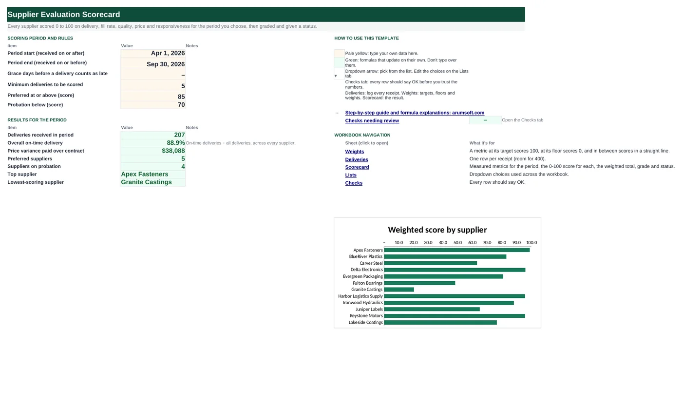
Supplier reviews go better with numbers both sides can check. This workbook keeps a log of every delivery (promised and received dates, quantities ordered, received and rejected, price paid and contract price) and turns it into on-time %, fill rate, defect rate and price variance for each supplier over the period you choose. Each metric becomes a 0–100 score between a target and a floor, the scores are weighted into one number, and every supplier gets a grade and a status.
- Sheets:
- 6
- Works with:
- Excel for Microsoft 365, Excel 2016 or later, Excel for Mac and Excel for the web
- Updated:
What you can do with it
- Delivery log with days late, an on-time flag (with optional grace days) and price variance per receipt
- Per-supplier on-time %, fill rate, defect rate and price variance for any date range, using SUMIFS and COUNTIFS
- Each metric scored 0–100 between your target and floor, weighted into one score, with a heat-map
- Letter grade (A+ to D) and Preferred / Approved / Probation status, with a score chart
What's inside
The workbook has 6 sheets. You only type on a few of them; the rest calculate.
| Sheet | What it's for | You enter | Calculated for you |
|---|---|---|---|
| Start Here | Period, rules and results | Period start and end, grace days, minimum deliveries, Preferred and Probation thresholds | Deliveries in period, overall on-time %, price variance paid, Preferred and Probation counts, top and lowest supplier |
| Weights | Targets, floors and weights | Target and floor per metric, weights, grade bands | Total weight |
| Deliveries | Receipt log (400) | PO date, supplier, PO, promised, received, quantities, price paid, contract price | Days late, in period, on time, price variance, spend at contract |
| Scorecard | One row per supplier (20) | Supplier, category, responsiveness rating 1–5 | Deliveries, on-time %, fill rate, defect rate, price variance, five scores, weighted score, grade, status |
| Lists | Categories | Supplier categories | Nothing |
| Checks | Six data checks | Nothing | OK or Review |
Before you start
- Export receipts from your purchasing system: PO, supplier, promised date, received date, quantities and prices.
- Agree targets with the team (and ideally the suppliers): what on-time and defect levels count as excellent and as unacceptable.
- Decide who rates responsiveness and how often; it is the one score that is a judgement.
Step-by-step guide
Pick the period
Start Here B6 and B7: receipts dated between these are scored. Set grace days (B8), the minimum deliveries for a fair score (B9) and the Preferred and Probation thresholds (B10, B11).
Set targets and weights
Weights tab: for each metric, the value that earns 100 and the value that earns 0, and how much it counts. Weights must total 100%.
List the suppliers
Scorecard columns A, B and I: name, category and a responsiveness rating from 1 to 5.
Log every receipt
Deliveries tab: one row per receipt. Leave Received blank for open orders; they are ignored until they arrive.
Read the scorecard
Measured metrics in E–H, scores in J–N, weighted score, grade and status in O–Q.
Review with suppliers
Share each supplier's row; the Deliveries tab filtered to that supplier is the evidence.
Formula map
Every formula in the workbook, grouped by the sheet and column it lives in. A column of copied formulas counts once; the range it covers is shown.
| Sheet | Cells | Functions | What it computes | Reads | Feeds |
|---|---|---|---|---|---|
| Deliveries | L5 copied down to row 404 | IF, AND | In the scoring period | E5 | Every scorecard SUMIFS uses it as a criterion, so changing the period re-scores everything. |
| Deliveries | M5 copied down to row 404 | IF | On time | E5, D5 | Summed per supplier for the on-time count. |
| Deliveries | N5 copied down to row 404 | IF | Price variance in dollars | I5, J5, G5 | Summed per supplier and divided by spend at contract for the price variance %. |
| Scorecard | C5 copied down to row 24 | IF, COUNTIFS | Deliveries in the period | A5 | Below the minimum on Start Here B9, the supplier shows "Not enough data". |
| Scorecard | F5 copied down to row 24 | IF, OR, SUMIFS | Fill rate | C5 | G5 (rejected ÷ received) and H5 (variance ÷ spend at contract) follow the same pattern. |
| Scorecard | J5 copied down to row 24 | IF, OR, ROUND, MAX, MIN | Metric score 0–100 | E5 | K5–N5 do the same for fill rate, defects, price and responsiveness. For defects and price the target is below the floor, and the same formula still works. |
| Scorecard | O5 copied down to row 24 | IF, OR, ROUND | Weighted score | J5, K5, L5, M5, N5 | Drives the grade, status and chart. |
| Scorecard | P5 copied down to row 24 | IF, LOOKUP | Letter grade | O5 | Shown next to the status. |
| Scorecard | Q5 copied down to row 24 | IF | Status | O5 | Counted on Start Here B18 and B19. |
| Start Here | B21 | IFERROR, INDEX, MATCH, MINIFS | Lowest-scoring supplier | — | The first conversation to have. |
Every formula, explained
Each formula below is copied straight from the file, so what you read here is exactly what the cell contains. Click any cell in Excel to see it in the formula bar.
=IF(E5="", 0, IF(AND(E5>='Start Here'!$B$6, E5<='Start Here'!$B$7),
    1, 0))
Returns 1 when the receipt date falls between the period start and end, 0 otherwise (including open orders).
Piece by piece
E5=""- Not received yet: 0.
AND(E5>='Start Here'!$B$6, E5<='Start Here'!$B$7)- Inside the period.
With the sample data: E5 = Jan 20, 2026 → L5 result 0
How it is used: Every scorecard SUMIFS uses it as a criterion, so changing the period re-scores everything.
How to change it: Change the dates on Start Here.
Learn this: How to Use AND and OR in Excel →=IF(E5="", "", IF(E5<=D5+'Start Here'!$B$8, 1, 0))1 if received on or before the promised date plus any grace days, otherwise 0.
Piece by piece
E5<=D5+'Start Here'!$B$8- Received by the promised date (+ grace).
With the sample data: E5 = Jan 20, 2026, D5 = Jan 20, 2026 → M5 result 1
How it is used: Summed per supplier for the on-time count.
How to change it: Set grace days on Start Here B8 (for example 1 for next-morning receipts).
Learn this: How to Use the IF Function in Excel →=IF(E5="", "", (I5-J5)*G5)What you paid over (or under) the contract price on the quantity received.
Piece by piece
(I5-J5)- Price paid minus contract price, per unit.
*G5- Times units received.
With the sample data: I5 = 50.57, J5 = 51.48, G5 = 200 → N5 result -182
How it is used: Summed per supplier and divided by spend at contract for the price variance %.
How to change it: Nothing to change.
Learn this: How to Write Basic Formulas in Excel →=IF(A5="", "", COUNTIFS(Deliveries!$B$5:$B$404,
A5, Deliveries!$L$5:$L$404,
1))Counts receipts for this supplier flagged as in period.
Piece by piece
Deliveries!$B$5:$B$404, A5- Supplier matches.
Deliveries!$L$5:$L$404, 1- In period.
With the sample data: A5 = Apex Fasteners → C5 result 20
How it is used: Below the minimum on Start Here B9, the supplier shows "Not enough data".
How to change it: Nothing to change.
Learn this: How to Use COUNTIF and COUNTIFS in Excel →=IF(OR(A5="", C5<'Start Here'!$B$9),
"", SUMIFS(Deliveries!$G$5:$G$404,
Deliveries!$B$5:$B$404, A5,
Deliveries!$L$5:$L$404, 1)/SUMIFS(Deliveries!$F$5:$F$404,
Deliveries!$B$5:$B$404, A5,
Deliveries!$L$5:$L$404, 1))Units received divided by units ordered, for this supplier's receipts in the period.
Piece by piece
SUMIFS(Deliveries!$G$5:$G$404, …)- Units received.
/SUMIFS(Deliveries!$F$5:$F$404, …)- Units ordered.
OR(A5="", C5<'Start Here'!$B$9)- Blank if too few deliveries.
With the sample data: C5 = 20 → F5 result 99.1%
How it is used: G5 (rejected ÷ received) and H5 (variance ÷ spend at contract) follow the same pattern.
How to change it: Nothing to change.
Learn this: How to Use SUMIF and SUMIFS in Excel →=IF(OR(A5="", E5=""), "",
ROUND(MAX(0, MIN(1, (E5-Weights!$C$5)/(Weights!$B$5-Weights!$C$5)))*100,
0))Places the measured value on a straight line between the floor (0) and the target (100), capped at both ends.
Piece by piece
(E5-Weights!$C$5)- Distance above the floor.
/(Weights!$B$5-Weights!$C$5)- As a share of the floor-to-target range.
MAX(0, MIN(1, …))- Never below 0 or above 1.
ROUND(…*100, 0)- Whole points.
With the sample data: E5 = 95.0% → J5 result 100
How it is used: K5–N5 do the same for fill rate, defects, price and responsiveness. For defects and price the target is below the floor, and the same formula still works.
How to change it: Change targets and floors on the Weights tab.
Learn this: How to Use MIN and MAX in Excel →=IF(OR(A5="", J5=""), "",
ROUND(J5*Weights!$D$5+K5*Weights!$D$6+L5*Weights!$D$7+M5*Weights!$D$8+N5*Weights!$D$9,
1))Each metric score times its weight, added up.
Piece by piece
J5*Weights!$D$5- On time × 30%.
+K5*Weights!$D$6 …- Fill 20%, quality 25%, price 15%, responsiveness 10%.
ROUND(…, 1)- One decimal.
With the sample data: J5 = 100, K5 = 100, L5 = 100, M5 = 92, N5 = 100 → O5 result 98.8
How it is used: Drives the grade, status and chart.
How to change it: Change the weights on the Weights tab.
Learn this: Relative, Absolute and Mixed References in Excel →=IF(O5="", "", LOOKUP(O5,
Weights!$A$13:$A$17, Weights!$B$13:$B$17))Approximate-match LOOKUP: finds the largest band start that is not above the score and returns its grade.
Piece by piece
LOOKUP(O5, Weights!$A$13:$A$17, Weights!$B$13:$B$17)- 0 D, 60 C, 70 B, 80 A, 90 A+.
With the sample data: O5 = 98.8 → P5 result A+
How it is used: Shown next to the status.
How to change it: Edit the bands on the Weights tab (keep them in ascending order).
Learn this: Lookup Formulas in Excel: XLOOKUP, VLOOKUP and INDEX/MATCH →=IF(A5="", "", IF(O5="", "Not enough data",
IF(O5>='Start Here'!$B$10, "Preferred", IF(O5<'Start Here'!$B$11, "Probation", "Approved"))))Not enough data without a score; Preferred at or above the Preferred threshold; Probation below the Probation threshold; otherwise Approved.
Piece by piece
O5=""- Too few deliveries.
O5>='Start Here'!$B$10- Preferred (85).
O5<'Start Here'!$B$11- Probation (70).
With the sample data: O5 = 98.8 → Q5 result Preferred
How it is used: Counted on Start Here B18 and B19.
How to change it: Change thresholds on Start Here.
Learn this: How to Use the IF Function in Excel →=IFERROR(INDEX(Scorecard!$A$5:$A$24,
MATCH(MINIFS(Scorecard!$O$5:$O$24, Scorecard!$O$5:$O$24, ">0"), Scorecard!$O$5:$O$24, 0)),
"")Finds the lowest score above zero (so unscored suppliers are skipped) and returns that supplier.
Piece by piece
MINIFS(Scorecard!$O$5:$O$24, Scorecard!$O$5:$O$24, ">0")- Lowest real score.
MATCH(…, 0)- Its row.
INDEX(Scorecard!$A$5:$A$24, …)- Supplier name.
With the sample data: B21 result Granite Castings
How it is used: The first conversation to have.
How to change it: Nothing to change.
Learn this: How to Use INDEX and MATCH in Excel →Tips and limits
- Capacity: 20 suppliers and 400 receipts. For more, extend the ranges with Ctrl+H ($404).
- Score a rolling period (the last 6 or 12 months) so one bad month does not define a supplier.
- Partial shipments: log each receipt as its own row with the quantity ordered on the first row only, or the fill rate will understate.
- Defect rate here is rejected ÷ received units. If you track PPM, multiply by 1,000,000.
- Share the targets with suppliers before you score them; a scorecard works best as a joint improvement tool.
Learn the skills behind this template
Was this guide helpful? Spot a mistake? Send feedback · admin@arumsoft.com