ABC Inventory Analysis Template for Excel
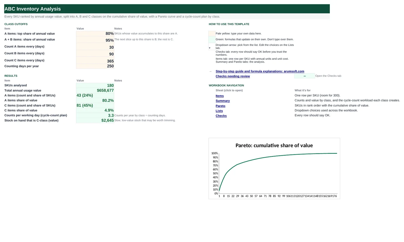
In most stockrooms a fifth of the items carry four-fifths of the value. ABC analysis finds them: multiply each SKU's annual units by its cost, rank the results, and split the list where the running total crosses 80% and 95%. This workbook does that for up to 300 SKUs, summarizes the classes, draws the Pareto curve and turns the classes into a cycle-count plan so the expensive items get counted most often.
- Sheets:
- 6
- Works with:
- Excel for Microsoft 365, Excel 2016 or later, Excel for Mac and Excel for the web
- Updated:
What you can do with it
- Annual usage value per SKU with a unique rank, even when two items tie
- Cumulative share of value and an A / B / C class from cutoffs you set (80% / 95% by default)
- Summary by class and by category: SKUs, value and share
- Pareto curve and a cycle-count plan: counts per year per class and counts per working day
What's inside
The workbook has 6 sheets. You only type on a few of them; the rest calculate.
| Sheet | What it's for | You enter | Calculated for you |
|---|---|---|---|
| Start Here | Cutoffs and the results | A cutoff, A+B cutoff, count interval per class, counting days per year | SKUs, total value, A and C counts and value shares, counts per working day, C-class stock on hand |
| Items | SKU list (300) | SKU, description, category, annual units, unit cost, on hand | Annual value, rank, share, cumulative share, class, on-hand value |
| Summary | By class and by category | Nothing | SKUs, share of SKUs, value, share of value, counts per year; A/B/C mix per category |
| Pareto | Items in rank order | Nothing | SKU, value, cumulative share and class for each rank |
| Lists | Categories | Category names | Nothing |
| Checks | Six data checks | Nothing | OK or Review |
Before you start
- Export 12 months of usage or sales quantity per SKU from your ERP or POS.
- Use the current standard or average cost per unit, not the selling price.
- Decide how often you can count: the plan turns your intervals into a daily counting workload.
Step-by-step guide
Set the cutoffs
Start Here B6 and B7: the share of value that makes an item A (80%) and the share for A plus B (95%).
Set the count intervals
Start Here B8–B11: days between counts for A, B and C items and the days a year you count.
Paste the items
Items tab: SKU, description, category, annual units, unit cost and units on hand. Value, rank, cumulative share and class calculate.
Read the summary
Summary tab: how many SKUs and how much value fall in each class, plus the class mix by category.
Look at the curve
Pareto tab and the Start Here chart: the steep part is your A items; where it flattens, the C items begin.
Plan the counts
Start Here B21 gives the counts per working day the plan needs. Set your cycle-count schedule by class.
Formula map
Every formula in the workbook, grouped by the sheet and column it lives in. A column of copied formulas counts once; the range it covers is shown.
| Sheet | Cells | Functions | What it computes | Reads | Feeds |
|---|---|---|---|---|---|
| Items | F5 copied down to row 304 | IF | Annual usage value | D5, E5 | Everything else ranks and adds this value. |
| Items | G5 copied down to row 304 | IF, RANK, COUNTIF | Unique rank | F5 | The cumulative share and the Pareto tab both need every rank to be different. |
| Items | I5 copied down to row 304 | IF, SUMIF | Cumulative share of value | G5 | The class is decided from it. |
| Items | J5 copied down to row 304 | IF | ABC class | I5, H5 | Colored by class; counted and summed on Summary. |
| Summary | D5 copied down to row 7 | SUMIF | Value by class | — | Divided by the total for the share of value. |
| Summary | G5 copied down to row 7 | arithmetic | Cycle counts per year | B5, F5 | The total ÷ counting days gives Start Here B21. |
| Summary | C11 copied down to row 20 | IF, COUNTIFS | Class mix by category | — | Shows which categories hold your high-value items. |
| Pareto | B5 copied down to row 304 | IFERROR, INDEX, MATCH | SKU at this rank | — | Columns C–E return value, cumulative share and class the same way, in rank order, for the curve. |
| Start Here | B22 | SUMIF | C-class stock on hand | — | A starting point for an excess-stock review. |
Every formula, explained
Each formula below is copied straight from the file, so what you read here is exactly what the cell contains. Click any cell in Excel to see it in the formula bar.
=IF(A5="", "", D5*E5)Annual units times unit cost: what the item is worth to you over a year.
Piece by piece
D5*E5- Units × cost.
IF(A5="", "", …)- Blank row stays blank.
With the sample data: D5 = 38, E5 = 9.95 → F5 result 378.1
How it is used: Everything else ranks and adds this value.
How to change it: Use usage value at cost, not sales at price.
Learn this: How to Write Basic Formulas in Excel →=IF(A5="", "", RANK(F5, $F$5:$F$304,
0)+COUNTIF($F$5:F5, F5)-1)Ranks the value from largest to smallest, then breaks ties by adding how many earlier rows had the same value.
Piece by piece
RANK(F5, $F$5:$F$304, 0)- Position by value, 1 = largest.
+COUNTIF($F$5:F5, F5)-1- Expanding range: 0 for the first of a tie, 1 for the second, and so on.
With the sample data: F5 = 378.1 → G5 result 140
How it is used: The cumulative share and the Pareto tab both need every rank to be different.
How to change it: Nothing to change.
Learn this: How to Use COUNTIF and COUNTIFS in Excel →=IF(A5="", "", SUMIF($G$5:$G$304,
"<="&G5, $F$5:$F$304)/'Start Here'!$B$16)Adds the value of every item ranked at or above this one and divides by the total.
Piece by piece
SUMIF($G$5:$G$304, "<="&G5, $F$5:$F$304)- Value of ranks 1 to this rank.
/'Start Here'!$B$16- Divided by total value.
With the sample data: G5 = 140 → I5 result 98.9%
How it is used: The class is decided from it.
How to change it: Nothing to change.
Learn this: How to Use SUMIF and SUMIFS in Excel →=IF(A5="", "", IF(I5-H5<'Start Here'!$B$6,
"A", IF(I5-H5<'Start Here'!$B$7, "B", "C")))Uses the share before this item (cumulative minus its own share), so the item that crosses the 80% line is still A.
Piece by piece
I5-H5- Cumulative share of the items ranked above.
<'Start Here'!$B$6- Under 80%: A.
<'Start Here'!$B$7- Under 95%: B.
"C"- Everything else.
With the sample data: I5 = 98.9%, H5 = 0.1% → J5 result C
How it is used: Colored by class; counted and summed on Summary.
How to change it: Change the cutoffs on Start Here.
Learn this: How to Use the IF Function in Excel →=SUMIF(Items!$J$5:$J$304, A5, Items!$F$5:$F$304)Adds the annual value of every item in class A (row 6 B, row 7 C).
Piece by piece
Items!$J$5:$J$304, A5- Class matches.
Items!$F$5:$F$304- Values to add.
With the sample data: D5 result 528,002.57
How it is used: Divided by the total for the share of value.
How to change it: Nothing to change.
Learn this: How to Use SUMIF and SUMIFS in Excel →=B5*F5SKUs in the class times how many times a year each is counted (365 ÷ the interval).
Piece by piece
B5- SKUs in class A.
F5 = 365/'Start Here'!$B$8- Counts per SKU per year.
With the sample data: B5 = 43, F5 = 12.17 → G5 result 523.17
How it is used: The total ÷ counting days gives Start Here B21.
How to change it: Change the intervals on Start Here.
Learn this: How to Write Basic Formulas in Excel →=IF(A11="", "", COUNTIFS(Items!$C$5:$C$304,
A11, Items!$J$5:$J$304, "A"))Counts the items that are both in this category and class A.
Piece by piece
Items!$C$5:$C$304, A11- Category matches.
Items!$J$5:$J$304, "A"- Class A (D11 and E11 use B and C).
With the sample data: C11 result 2
How it is used: Shows which categories hold your high-value items.
How to change it: Nothing to change.
Learn this: How to Use COUNTIF and COUNTIFS in Excel →=IFERROR(INDEX(Items!$A$5:$A$304,
MATCH(A5, Items!$G$5:$G$304, 0)),
"")Looks up which item has rank 1 (2, 3 …) and returns its code.
Piece by piece
MATCH(A5, Items!$G$5:$G$304, 0)- Row of the item with this rank.
INDEX(Items!$A$5:$A$304, …)- Its SKU.
IFERROR(…, "")- Blank past the last item.
With the sample data: B5 result SKU-1108
How it is used: Columns C–E return value, cumulative share and class the same way, in rank order, for the curve.
How to change it: Nothing to change.
Learn this: How to Use INDEX and MATCH in Excel →=SUMIF(Items!$J$5:$J$304, "C", Items!$K$5:$K$304)Adds the on-hand value of every C item: slow, low-value stock that may be worth trimming.
Piece by piece
Items!$J$5:$J$304, "C"- Class C.
Items!$K$5:$K$304- On-hand value.
With the sample data: B22 result 2,644.63
How it is used: A starting point for an excess-stock review.
How to change it: Change "C" to "A" to see what your A items tie up.
Learn this: How to Use SUMIF and SUMIFS in Excel →Tips and limits
- Capacity: 300 SKUs. Extend by inserting rows inside the Items table and the Pareto tab, then copy the formulas down.
- Rerun the analysis every quarter. Items move between classes as demand changes.
- Value is not the only criterion. Promote a cheap item to A if running out stops the line (critical spares, safety items).
- Cutoffs of 70/90 or 80/95 are both common; pick one and keep it so trends are comparable.
- The Pareto chart plots only the rows with data; it updates when you add items.
Learn the skills behind this template
Was this guide helpful? Spot a mistake? Send feedback · admin@arumsoft.com