Petty Cash Reconciliation Log for Excel
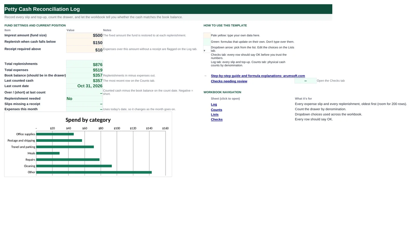
An imprest petty cash fund is simple to run when the log does the arithmetic: every slip reduces the running balance, every top-up restores it to the fund size, and a cash count by denomination tells you in one cell whether the drawer is over or short. The workbook also flags slips over your receipt threshold with no receipt and totals spend by category for the journal entry.
- Sheets:
- 5
- Works with:
- Excel for Microsoft 365, Excel 2016 or later, Excel for Mac and Excel for the web
- Updated:
What you can do with it
- Running balance after every slip and replenishment
- Cash count by denomination with over/short against the book balance on that date
- Receipt-required flags and a replenishment prompt when cash falls below your threshold
- Spend by category for the month-end journal entry
What's inside
The workbook has 5 sheets. You only type on a few of them; the rest calculate.
| Sheet | What it's for | You enter | Calculated for you |
|---|---|---|---|
| Start Here | Fund settings and current position | Imprest amount, replenish-below threshold, receipt threshold | Replenishments, expenses, book balance, last count, over/short, replenishment needed, missing receipts, expenses this month |
| Log | Every slip and top-up (room for 200) | Date, type, payee, category, amount out, reference, taken by, receipt?, amount in | Flag, running balance, spend by category |
| Counts | Cash counts by denomination (12) | Count date, counted by, number of each bill and coin | Cash counted, book balance on that date, over/short, status |
| Lists | Dropdowns | Types, categories, receipt yes/no | Nothing |
| Checks | Six data checks | Nothing | OK or Review |
Before you start
- Decide the fund size (the imprest amount) and the balance at which you will replenish. $300–$1,000 is typical for a small office.
- Decide the receipt rule: above what amount is a receipt mandatory?
- Gather the slips since the last reconciliation, in date order.
Step-by-step guide
Set the fund rules
Start Here B6 imprest amount, B7 replenish-below threshold, B8 receipt-required threshold.
Log the opening float
Log row 5: type Replenishment, amount in = the imprest amount. The running balance starts there.
Record every slip
Date, Expense, payee, category (dropdown), amount out, slip number, who took the cash, and whether a receipt is attached. The running balance and the flag column update.
Replenish
Add a Replenishment row. In the sample, Amount in is a formula (imprest amount minus the previous balance) so the fund returns to exactly the fund size; type over it if the deposit differs.
Count the drawer
Counts tab: date, who counted, and how many of each bill and coin. Cash counted, the book balance on that date and the over/short calculate.
Read Start Here and check
Book balance, last count, over/short and whether a replenishment is due. The Checks tab catches out-of-order dates, a negative balance, uncategorized slips, flagged slips, an unbalanced count, and a book balance above the fund size.
Formula map
Every formula in the workbook, grouped by the sheet and column it lives in. A column of copied formulas counts once; the range it covers is shown.
| Sheet | Cells | Functions | What it computes | Reads | Feeds |
|---|---|---|---|---|---|
| Log | K6 copied down to row 204 | IF | Running balance | K5, I6, E6 | Start Here B12 recomputes the same thing from totals; the Counts tab uses date-bounded sums instead. |
| Log | I14 copied down to row 32 | arithmetic | Replenishment to the imprest amount | K13 | Keeps the sample balanced; in real use, type the deposit amount if it differs. |
| Log | J6 copied down to row 204 | IF, AND | Flag | B6, E6, H6 | Counted on Start Here B17 and on the Checks tab. |
| Counts | M5 copied down to row 16 | IF, SUMPRODUCT | Cash counted | — | Compared with the book balance for over/short. |
| Counts | N5 copied down to row 16 | IF, SUMIFS | Book balance on the count date | A5 | What should be in the drawer when the count is taken. |
| Counts | P5 copied down to row 16 | IF, ABS | Status | O5 | Conditional formatting colors the three states. |
| Start Here | B13 | IFERROR, LOOKUP | Last counted cash | — | B14 and B15 use the same pattern for the date and over/short. |
| Start Here | B16 | IF, TEXT | Replenishment needed | B12, B7, B6 | A plain-language prompt on the dashboard. |
| Start Here | B18 | SUMIFS, DATE, YEAR, TODAY, MONTH | Expenses this month | — | Changes every day; the sample shows 0 because its dates are in the past. |
| Log | N5 copied down to row 11 | IF, SUMIF | Spend by category | — | The journal entry at replenishment: debit each category, credit cash. Charted on Start Here. |
Every formula, explained
Each formula below is copied straight from the file, so what you read here is exactly what the cell contains. Click any cell in Excel to see it in the formula bar.
=IF(A6="", "", K5+I6-E6)The previous balance plus money in minus money out. Row 5 starts from its own amount in.
Piece by piece
K5- Previous running balance.
+I6- Replenishment amount (blank for expenses).
-E6- Expense amount (blank for replenishments).
With the sample data: K5 = 500, I6 = —, E6 = 13.8 → K6 result 486.2
How it is used: Start Here B12 recomputes the same thing from totals; the Counts tab uses date-bounded sums instead.
How to change it: Nothing to change.
Learn this: How to Write Basic Formulas in Excel →='Start Here'!$B$6-K13In the sample, each top-up is the fund size minus the balance just before it, so the fund returns to exactly the imprest amount.
Piece by piece
'Start Here'!$B$6- Fund size.
-K13- Running balance on the previous row.
With the sample data: K13 = 347.71 → I14 result 152.29
How it is used: Keeps the sample balanced; in real use, type the deposit amount if it differs.
How to change it: Type a number over it.
Learn this: Relative, Absolute and Mixed References in Excel →=IF(A6="", "", IF(AND(B6="Expense", E6>'Start Here'!$B$8, H6<>"Yes"),
"Missing receipt", IF(AND(B6="Expense", E6=0), "No amount", "")))Marks an expense over the receipt threshold that has no receipt, and an expense with no amount.
Piece by piece
B6="Expense"- Only expenses are tested.
E6>'Start Here'!$B$8- Above the threshold.
H6<>"Yes"- Receipt not marked Yes.
E6=0- An expense row with nothing in Amount out.
With the sample data: B6 = Expense, E6 = 13.8, H6 = Yes → J6 result —
How it is used: Counted on Start Here B17 and on the Checks tab.
How to change it: Add other tests inside the nested IF.
Learn this: How to Use AND and OR in Excel →=IF(A5="", "", SUMPRODUCT(C5:L5, $C$3:$L$3))Multiplies the number of each bill and coin by its face value in row 3 and adds them up.
Piece by piece
C5:L5- How many of each denomination.
$C$3:$L$3- Face values: $100 down to 1¢.
SUMPRODUCT(…)- Multiply pairs and add.
With the sample data: M5 result 347.71
How it is used: Compared with the book balance for over/short.
How to change it: To add a $2 bill or a different currency, change the face values in row 3.
Learn this: How to Use SUMIF and SUMIFS in Excel →=IF(A5="", "", SUMIFS(Log!$I$5:$I$204,
Log!$A$5:$A$204, "<="&A5)-SUMIFS(Log!$E$5:$E$204,
Log!$A$5:$A$204, "<="&A5))Replenishments up to and including the count date minus expenses up to that date. Dates are compared as text criteria ("<="&date).
Piece by piece
SUMIFS(Log!$I$5:$I$204, Log!$A$5:$A$204, "<="&A5)- Money in through the count date.
-SUMIFS(Log!$E$5:$E$204, …)- Money out through the count date.
With the sample data: A5 = Jul 31, 2026 → N5 result 347.71
How it is used: What should be in the drawer when the count is taken.
How to change it: Nothing to change.
Learn this: How to Use SUMIF and SUMIFS in Excel →=IF(A5="", "", IF(ABS(O5)<0.005,
"Balanced", IF(O5>0, "Over", "Short")))Balanced when the difference is under half a cent, otherwise Over or Short.
Piece by piece
ABS(O5)<0.005- Difference rounds to zero.
O5>0- Counted more than the book: Over.
With the sample data: O5 = 0 → P5 result Balanced
How it is used: Conditional formatting colors the three states.
How to change it: Change 0.005 to tolerate small rounding differences.
Learn this: How to Use the IF Function in Excel →=IFERROR(LOOKUP(2, 1/(Counts!$A$5:$A$16<>""),
Counts!$M$5:$M$16), 0)Returns the cash counted on the last non-blank row of the Counts tab. LOOKUP(2, 1/(range<>""), …) is the classic "last value" trick: 1 divided by TRUE gives 1, by FALSE gives an error, and LOOKUP returns the last 1 it finds.
Piece by piece
Counts!$A$5:$A$16<>""- TRUE on rows with a count date.
1/(…)- 1 on those rows, #DIV/0! elsewhere.
LOOKUP(2, …, Counts!$M$5:$M$16)- Searches for 2, never finds it, and returns the value next to the last 1.
With the sample data: B13 result 357.13
How it is used: B14 and B15 use the same pattern for the date and over/short.
How to change it: Nothing to change.
Learn this: Lookup Formulas in Excel: XLOOKUP, VLOOKUP and INDEX/MATCH →=IF(B12<B7, "Yes — "&TEXT(B6-B12,
"$#, ##0")&" to restore",
"No")If the book balance is below the threshold, builds a message with the amount needed to restore the fund.
Piece by piece
B12<B7- Below the threshold.
TEXT(B6-B12, "$#,##0")- Fund size minus balance, formatted as currency.
"Yes — "&…&" to restore"- Joined into a message.
With the sample data: B12 = 357.13, B7 = 150, B6 = 500 → B16 result No
How it is used: A plain-language prompt on the dashboard.
How to change it: Nothing to change.
Learn this: Text and Date Functions in Excel →=SUMIFS(Log!$E$5:$E$204, Log!$A$5:$A$204,
">="&DATE(YEAR(TODAY()),
MONTH(TODAY()), 1))Adds expenses dated on or after the first day of the current month.
Piece by piece
DATE(YEAR(TODAY()), MONTH(TODAY()), 1)- The first of this month.
">="&…- Criterion: on or after.
SUMIFS(Log!$E$5:$E$204, Log!$A$5:$A$204, …)- Expenses meeting it.
With the sample data: B18 result 0
How it is used: Changes every day; the sample shows 0 because its dates are in the past.
How to change it: Nothing to change.
Learn this: How to Use TODAY and NOW in Excel →=IF(M5="", "", SUMIF($D$5:$D$204, M5, $E$5:$E$204))Adds expenses whose category matches the label in column M, pulled from the Lists tab.
Piece by piece
$D$5:$D$204- Category column.
M5- The category.
$E$5:$E$204- Amounts.
With the sample data: N5 result 46.42
How it is used: The journal entry at replenishment: debit each category, credit cash. Charted on Start Here.
How to change it: Nothing to change; add categories on the Lists tab.
Learn this: How to Use SUMIF and SUMIFS in Excel →Tips and limits
- Capacity: 200 log rows, 12 counts. Start a new file each year, carrying the final running balance in as the opening replenishment.
- Reconcile before every replenishment: cash counted + slips since the last top-up should equal the fund size. The Counts tab shows the gap.
- Small, repeated shortages are worth a conversation; one-off cents are usually rounding at the register.
- Keep the slips with the count sheet. The Reference column (slip or check number) is what the auditor matches to paper.
- If you keep multiple funds, use one copy of the file per fund; the Start Here settings are per fund.
Learn the skills behind this template
Was this guide helpful? Spot a mistake? Send feedback · admin@arumsoft.com