Recipe Costing and Plate Margin Calculator for Excel
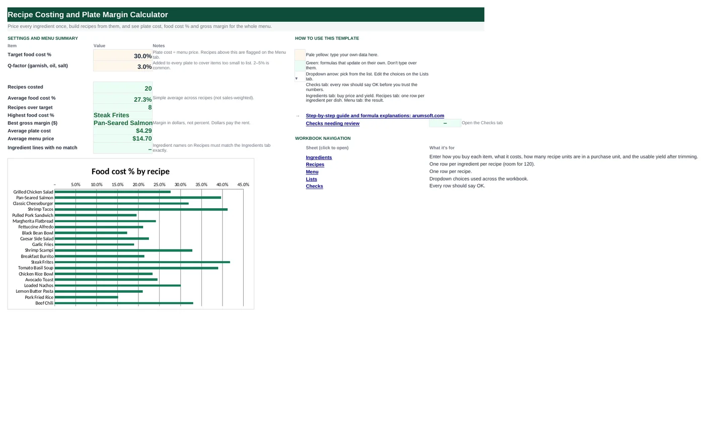
Price each ingredient once, with the purchase unit, the recipe unit and the usable yield after trimming. Build each recipe as a list of ingredient lines; the workbook looks up the cost per unit, adds a Q-factor for garnish and seasoning, and puts every menu item on one page with plate cost, food cost %, gross margin in dollars and the price that would hit your target. Twenty sample recipes come in the file.
- Sheets:
- 6
- Works with:
- Excel for Microsoft 365, Excel 2016 or later, Excel for Mac and Excel for the web
- Updated:
Recipe Costing and Plate Margin Calculator.xlsx
Free to download. No sign-up needed.
What you can do with it
- Cost per recipe unit from purchase price, pack size and yield
- Recipes built from ingredient lines with INDEX/MATCH lookups
- Plate cost, food cost %, gross margin and price at target for every menu item
- A food cost % chart and six checks that catch unmatched ingredients and missing prices
What's inside
The workbook has 6 sheets. You only type on a few of them; the rest calculate.
| Sheet | What it's for | You enter | Calculated for you |
|---|---|---|---|
| Start Here | Targets and the menu summary | Target food cost %, Q-factor | Recipes costed, average food cost %, recipes over target, highest food cost item, best margin item, average plate cost and price, unmatched lines |
| Ingredients | One row per ingredient (60) | Name, category, purchase unit and price, recipe unit, units per purchase, yield %, date | Cost per recipe unit |
| Recipes | One row per ingredient per recipe (120) | Recipe, ingredient, quantity | Unit, unit cost, line cost, lookup status |
| Menu | One row per menu item (20) | Recipe, category, servings, menu price | Ingredient cost, Q-factor, plate cost, food cost %, gross margin, price at target, status |
| Lists | Dropdowns | Categories, units, menu categories | Nothing |
| Checks | Six data checks | Nothing | OK or Review |
Before you start
- Gather current invoices for your main ingredients: the pack you buy and what it costs.
- Decide the recipe unit for each (oz, each, fl oz) and how many of those are in a pack. Estimate yield for anything you trim or peel.
- Write each recipe as ingredient and quantity per plate (or per batch, then set the servings on the Menu tab).
Step-by-step guide
Set the targets
Start Here B6 is the target food cost %; B7 is the Q-factor added to every plate for garnish, oil and seasoning you do not list (2–5%).
Price the ingredients
Ingredients tab: how you buy it, what it costs, the recipe unit, how many recipe units are in a purchase unit, and the yield. Cost per recipe unit calculates.
Build the recipes
Recipes tab: recipe name (dropdown from the Menu tab), ingredient (dropdown), quantity. Unit and cost are looked up; a "Not found" lookup means the name does not match the Ingredients tab.
Set menu prices
Menu tab: one row per item with category, servings per recipe and the price. Plate cost, food cost %, margin and the price at target calculate.
Read Start Here
Which items are over target, which has the highest food cost %, which earns the most margin in dollars, and the average plate cost and price. The chart ranks food cost % by recipe.
Fix what the Checks tab flags
Unmatched ingredient names, ingredients without a cost, duplicate names, menu items without a price or without recipe lines, and yields outside 50–100%.
Formula map
Every formula in the workbook, grouped by the sheet and column it lives in. A column of copied formulas counts once; the range it covers is shown.
| Sheet | Cells | Functions | What it computes | Reads | Feeds |
|---|---|---|---|---|---|
| Ingredients | H5 copied down to row 64 | IF, OR | Cost per recipe unit | D5, F5, G5 | Looked up by every recipe line. |
| Recipes | E5 copied down to row 124 | IF, IFERROR, INDEX, MATCH | Unit cost lookup | B5 | Line cost multiplies this by quantity. |
| Recipes | G5 copied down to row 124 | IF, ISNUMBER, MATCH | Lookup status | B5 | Counted on Start Here B16 and on the Checks tab. |
| Menu | D5 copied down to row 24 | IF, SUMIF | Ingredient cost per serving | C5 | The base for plate cost. |
| Menu | F5 copied down to row 24 | IF | Plate cost | D5, E5 | Food cost %, margin and price at target all start here. |
| Menu | H5 copied down to row 24 | IF, OR | Food cost % | F5, G5 | Compared with the target for the status; charted on Start Here. |
| Menu | J5 copied down to row 24 | IF | Price at target | F5 | Compare with what you charge today; a large gap is a pricing decision or a recipe to rework. |
| Menu | K5 copied down to row 24 | IF | Status | H5 | Conditional formatting colors the three states. |
| Start Here | B13 | IFERROR, INDEX, MATCH, MAX | Best gross margin | — | Dollars matter more than percent: a 40% food cost on a $28 plate earns more than 20% on a $7 side. |
| Checks | B7 | IF, SUMPRODUCT, COUNTIF | Ingredient names are unique | — | A silent wrong lookup is the hardest error to spot. |
Every formula, explained
Each formula below is copied straight from the file, so what you read here is exactly what the cell contains. Click any cell in Excel to see it in the formula bar.
=IF(OR(A5="", F5=0, G5=0), "", D5/F5/G5)Purchase price divided by the number of recipe units in a pack, then divided by yield so the cost of the trimmed-away part is carried by what you serve.
Piece by piece
OR(A5="", F5=0, G5=0)- Blank row or missing pack size or yield: show nothing.
D5/F5- Price per recipe unit before yield.
/G5- Divided by yield (0.9 = 90% usable) raises the usable cost.
With the sample data: D5 = 4.14, F5 = 1, G5 = 95.0% → H5 result 4.36
How it is used: Looked up by every recipe line.
How to change it: Nothing to change.
Learn this: How to Write Basic Formulas in Excel →=IF(B5="", "", IFERROR(INDEX(Ingredients!$H$5:$H$64, MATCH(B5, Ingredients!$A$5:$A$64, 0)),
0))Finds the ingredient on the Ingredients tab and returns its cost per recipe unit.
Piece by piece
MATCH(B5, Ingredients!$A$5:$A$64, 0)- Row number of the ingredient (exact match).
INDEX(Ingredients!$H$5:$H$64, …)- The cost on that row.
IFERROR(…, 0)- Zero if the name is not found, so the line cost does not error.
With the sample data: B5 = Chicken breast → E5 result 4.36
How it is used: Line cost multiplies this by quantity.
How to change it: Nothing to change.
Learn this: How to Use INDEX and MATCH in Excel →=IF(B5="", "", IF(ISNUMBER(MATCH(B5, Ingredients!$A$5:$A$64, 0)),
"OK", "Not found"))Shows whether the ingredient name matches the Ingredients tab, so a zero cost from a typo is visible.
Piece by piece
MATCH(B5, Ingredients!$A$5:$A$64, 0)- A number if found, an error if not.
ISNUMBER(…)- TRUE when found.
With the sample data: B5 = Chicken breast → G5 result OK
How it is used: Counted on Start Here B16 and on the Checks tab.
How to change it: Nothing to change.
Learn this: How to Use IFERROR in Excel →=IFERROR(INDEX(Menu!$A$5:$A$24,
MATCH(MAX(Menu!$I$5:$I$24), Menu!$I$5:$I$24, 0)),
"")Finds the largest margin in dollars on the Menu tab and returns the item name.
Piece by piece
MAX(Menu!$I$5:$I$24)- Largest gross margin.
MATCH(…, Menu!$I$5:$I$24, 0)- Its row.
INDEX(Menu!$A$5:$A$24, …)- The item on that row.
With the sample data: B13 result Pan-Seared Salmon
How it is used: Dollars matter more than percent: a 40% food cost on a $28 plate earns more than 20% on a $7 side.
How to change it: Nothing to change.
Learn this: How to Use INDEX and MATCH in Excel →=IF(SUMPRODUCT((Ingredients!$A$5:$A$64<>"")*(COUNTIF(Ingredients!$A$5:$A$64, Ingredients!$A$5:$A$64)>1))=0,
"OK", "Review")A duplicate name would make the lookup return the first one silently, so this counts how many names appear more than once.
Piece by piece
COUNTIF(Ingredients!$A$5:$A$64, Ingredients!$A$5:$A$64)>1- TRUE for any name that appears twice or more.
(Ingredients!$A$5:$A$64<>"")*…- Ignore blank rows.
SUMPRODUCT(…)=0- No duplicates.
With the sample data: B7 result OK
How it is used: A silent wrong lookup is the hardest error to spot.
How to change it: Nothing to change.
Learn this: How to Use COUNTIF and COUNTIFS in Excel →Tips and limits
- Capacity: 60 ingredients, 120 recipe lines, 20 menu items. For more, extend the ranges with Ctrl+H ($64, $124, $24).
- Re-price ingredients monthly from the latest invoices; the Last updated column shows what is stale. Every plate cost updates at once.
- The Q-factor replaces listing salt, oil and garnish on every recipe. If you do list them, set it to 0.
- Price at target is a starting point, not a rule. Use the margin-in-dollars column alongside it: the goal is dollars per seat, not a percentage.
- For batch recipes (soups, sauces), enter the whole batch on the Recipes tab and set Servings on the Menu tab to the number of portions it yields.
Learn the skills behind this template
Was this guide helpful? Spot a mistake? Send feedback · admin@arumsoft.com