Tiered Sales Commission Calculator for Excel
Log deals, set quotas and define up to four attainment tiers; the workbook works out each rep's attainment, pays every slice of it at the right tier rate (or everything at the tier reached, if that is your plan), adds SPIFFs, and totals the payout for the period. The tier columns on the Reps tab show exactly how each number was built, which is what reps ask to see.
- Sheets:
- 6
- Works with:
- Excel for Microsoft 365, Excel 2016 or later, Excel for Mac and Excel for the web
- Updated:
What you can do with it
- Compute attainment per rep from a deal log for any period
- Pay accelerator tiers marginally (each slice at its rate) or flat (all at the tier reached)
- Add SPIFFs and bonuses by rep
- Get the period payout and blended rate for the accrual
What's inside
The workbook has 6 sheets. You only type on a few of them; the rest calculate.
| Sheet | What it's for | You enter | Calculated for you |
|---|---|---|---|
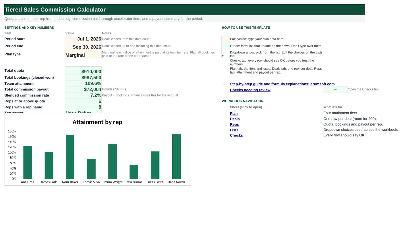
| Start Here | Period, plan type and the payout summary | Period start and end, plan type | Total quota, bookings, attainment, payout, blended rate, reps at quota, top earner |
| Plan | The four tiers and the SPIFF list | Tier boundaries and rates; SPIFFs by rep | Example payout at the top of each tier |
| Deals | One row per deal (room for 200) | Close date, rep, account, amount, stage | In period?, Counts? |
| Reps | Attainment and payout per rep (30) | Rep, role, quota | Bookings, attainment, tier reached, pay per tier, marginal and flat payout, total, effective rate |
| Lists | Dropdowns | Rep names, stages, plan types, roles | Nothing |
| Checks | Six plan and data checks | Nothing | OK or Review |
Before you start
- Write down your plan as tiers: attainment from, attainment to, rate. The sample is 4% to 50%, 8% to 100%, 12% to 150%, 15% above.
- Decide whether tiers are marginal (the usual accelerator) or flat (retroactive to the first dollar). The Start Here dropdown switches the whole workbook.
- Export closed deals for the period with close date, rep, amount and stage.
Step-by-step guide
Set the period and plan type
Start Here B6 and B7 bound the period; only deals closed inside it count. B8 picks Marginal or Flat.
Define the tiers on the Plan tab
Rows 5–8: attainment from, to and the rate. Keep the tiers contiguous and the top tier open-ended (to = 1000%). Column E shows what a $100,000 quota would pay at the top of each tier, a quick sanity check for the plan.
Add SPIFFs
Plan rows 14–23: rep, amount and reason. They are added to the rep's total on the Reps tab regardless of attainment.
Enter deals
Deals tab: close date, rep (dropdown), account, amount, stage. The two calculated columns show whether the deal is in the period and whether it counts (in period and Closed Won).
Set quotas on the Reps tab
One row per rep with role and quota for the period. Bookings, attainment and the tier reached calculate; the four tier columns show the marginal payout piece by piece; the total applies the plan type and adds SPIFFs.
Read the Start Here summary
Total payout and the blended rate are what finance needs for the accrual; reps at or above quota and the top earner are for the sales meeting.
Check the Checks tab
Catches non-contiguous tiers, a capped top tier, a deal rep missing from Lists, a rep without a quota, and a mismatch between the tier columns and the marginal total.
Formula map
Every formula in the workbook, grouped by the sheet and column it lives in. A column of copied formulas counts once; the range it covers is shown.
| Sheet | Cells | Functions | What it computes | Reads | Feeds |
|---|---|---|---|---|---|
| Deals | G5 copied down to row 204 | IF, AND | Does the deal count? | F5, E5 | The Reps tab sums amounts where this column says Yes. |
| Reps | D5 copied down to row 34 | IF, SUMIFS | Bookings per rep | — | Attainment divides this by quota. |
| Reps | E5 copied down to row 34 | IF, OR | Attainment | D5, C5 | Every tier column compares against this. |
| Reps | F5 copied down to row 34 | IF, MATCH | Tier reached | E5 | The flat payout uses this to pick a rate. |
| Reps | G5 copied down to row 34 | IF, MAX, MIN | Pay within one tier | E5, C5 | K5 adds the four tier columns. |
| Reps | L5 copied down to row 34 | IF, INDEX | Flat payout | D5, F5 | Used when Start Here B8 is Flat. |
| Reps | M5 copied down to row 34 | IF, SUMIF | Total payout | K5, L5 | Summed on Start Here B13. |
| Plan | E5 copied down to row 8 | SUMPRODUCT | Example payout at the top of a tier | — | A sanity check when designing the plan. |
| Start Here | B14 | IF | Blended commission rate | B13, B11 | Compare with the plan's base rate to see what accelerators and SPIFFs are costing. |
| Checks | B6 | IF, AND | Tiers are contiguous | — | A gap or overlap would pay too little or too much for the attainment in between. |
Every formula, explained
Each formula below is copied straight from the file, so what you read here is exactly what the cell contains. Click any cell in Excel to see it in the formula bar.
=IF(A5="", "", IF(AND(F5="Yes", E5="Closed Won"),
    "Yes", "No"))
A deal counts toward attainment only when it closed inside the period and its stage is Closed Won.
Piece by piece
F5="Yes"- In period (column F compares the close date with Start Here B6 and B7).
E5="Closed Won"- Stage test; exact spelling matters.
AND(…)- Both must be true.
With the sample data: F5 = Yes, E5 = Closed Won → G5 result Yes
How it is used: The Reps tab sums amounts where this column says Yes.
How to change it: To count Closed Won and Invoiced, use OR(E5="Closed Won",E5="Invoiced").
Learn this: How to Use AND and OR in Excel →=IF(A5="", "", SUMIFS(Deals!$D$5:$D$204,
Deals!$B$5:$B$204, A5, Deals!$G$5:$G$204,
"Yes"))Adds deal amounts for the rep where the deal counts.
Piece by piece
Deals!$D$5:$D$204- Amounts to sum.
Deals!$B$5:$B$204, A5- Rep matches.
Deals!$G$5:$G$204, "Yes"- The Counts? flag.
With the sample data: D5 result 188,000
How it is used: Attainment divides this by quota.
How to change it: Nothing to change.
Learn this: How to Use SUMIF and SUMIFS in Excel →=IF(OR(A5="", C5=0), "", D5/C5)Bookings divided by quota, as a fraction (1.25 = 125%).
Piece by piece
OR(A5="", C5=0)- No rep or no quota: show nothing rather than divide by zero.
D5/C5- Bookings ÷ quota.
With the sample data: D5 = 188,000, C5 = 150,000 → E5 result 1.25
How it is used: Every tier column compares against this.
How to change it: Nothing to change.
Learn this: How to Write Basic Formulas in Excel →=IF(E5="", "", MATCH(E5, Plan!$B$5:$B$8, 1))MATCH with match type 1 finds the last tier whose "from" is less than or equal to the attainment. The Plan tab's "from" column must be sorted ascending, which contiguous tiers guarantee.
Piece by piece
E5- Attainment.
Plan!$B$5:$B$8- The "from" boundaries: 0%, 50%, 100%, 150%.
1- Approximate match: largest value ≤ attainment.
With the sample data: E5 = 1.25 → F5 result 3
How it is used: The flat payout uses this to pick a rate.
How to change it: Nothing to change.
Learn this: How to Use INDEX and MATCH in Excel →=IF($E5="", "", $C5*Plan!$D$5*MAX(0,
MIN($E5, Plan!$C$5)-Plan!$B$5))The slice of attainment that falls inside the tier, times quota, times the tier rate. Columns H, I and J are identical except they point at Plan rows 6, 7 and 8.
Piece by piece
MIN($E5, Plan!$C$5)- Attainment capped at the tier's top.
-Plan!$B$5- Minus the tier's bottom: the width of attainment inside this tier.
MAX(0, …)- Zero if the rep never reached this tier.
$C5*Plan!$D$5*…- Quota × rate × that width = dollars paid for this tier.
With the sample data: E5 = 1.25, C5 = 150,000 → G5 result 3,000
How it is used: K5 adds the four tier columns.
How to change it: For a fifth tier, add a Plan row and a column with the same pattern pointing at row 9.
Learn this: How to Use MIN and MAX in Excel →=IF(E5="", "", D5*INDEX(Plan!$D$5:$D$8, F5))All bookings paid at the rate of the tier reached. INDEX picks the rate by tier number.
Piece by piece
INDEX(Plan!$D$5:$D$8, F5)- The rate on the row of the tier reached.
D5*…- Bookings × that rate.
With the sample data: D5 = 188,000, F5 = 3 → L5 result 22,560
How it is used: Used when Start Here B8 is Flat.
How to change it: Nothing to change.
Learn this: How to Use INDEX and MATCH in Excel →=IF(E5="", "", IF('Start Here'!$B$8="Flat",
L5, K5)+SUMIF(Plan!$A$14:$A$23,
A5, Plan!$B$14:$B$23))Marginal or flat payout depending on the plan type, plus any SPIFFs for the rep.
Piece by piece
'Start Here'!$B$8="Flat"- Plan type test.
L5 / K5- Flat or marginal payout.
SUMIF(Plan!$A$14:$A$23, A5, Plan!$B$14:$B$23)- SPIFF amounts whose rep matches.
With the sample data: K5 = 13,560, L5 = 22,560 → M5 result 13,560
How it is used: Summed on Start Here B13.
How to change it: Nothing to change.
Learn this: How to Use the IF Function in Excel →=SUMPRODUCT(100000*$D$5:D5*($C$5:C5-$B$5:B5))For a $100,000 quota, the pay accumulated through the end of this tier: each tier's width × rate, summed from tier 1 to this row. The expanding range ($D$5:D5) grows as the formula is copied down.
Piece by piece
$C$5:C5-$B$5:B5- Width of every tier up to this one.
100000*$D$5:D5*…- Quota × rate × width for each.
SUMPRODUCT(…)- Adds them.
With the sample data: E5 result 2,000
How it is used: A sanity check when designing the plan.
How to change it: Change 100000 to your typical quota.
Learn this: How to Use SUMIF and SUMIFS in Excel →=IF(B11=0, 0, B13/B11)Total payout divided by total bookings: the percentage finance accrues against revenue.
Piece by piece
B11=0- No bookings: show 0.
B13/B11- Payout ÷ bookings.
With the sample data: B13 = 72,004, B11 = 997,500 → B14 result 7.2%
How it is used: Compare with the plan's base rate to see what accelerators and SPIFFs are costing.
How to change it: Nothing to change.
Learn this: How to Write Basic Formulas in Excel →=IF(AND(Plan!$B$5=0, Plan!$B$6=Plan!$C$5,
Plan!$B$7=Plan!$C$6, Plan!$B$8=Plan!$C$7),
"OK", "Review")Each tier must start exactly where the previous one ended, and the first must start at 0%.
Piece by piece
Plan!$B$5=0- First tier starts at zero.
Plan!$B$6=Plan!$C$5- Tier 2 starts where tier 1 ends (and so on for 3 and 4).
AND(…)- All four tests must pass.
With the sample data: B6 result OK
How it is used: A gap or overlap would pay too little or too much for the attainment in between.
How to change it: Nothing to change.
Learn this: How to Use AND and OR in Excel →Tips and limits
- Capacity: 30 reps, 200 deals, 4 tiers, 10 SPIFF rows. For more deals, use Ctrl+H on formulas to replace $204 with a larger row.
- Marginal tiers reward every extra dollar without cliffs; flat (retroactive) tiers create a strong push at each boundary and a bigger cost. The workbook shows both columns so you can compare plans before choosing.
- Deals in the Open stage are ignored; change the stage to Closed Won when the contract is signed, not when the forecast says so.
- For a quarterly plan with monthly payouts, keep one copy per month and set the period to the month; attainment then resets each month.
Learn the skills behind this template
Was this guide helpful? Spot a mistake? Send feedback · admin@arumsoft.com