SaaS Cohort Retention and Net Dollar Retention Matrix for Excel
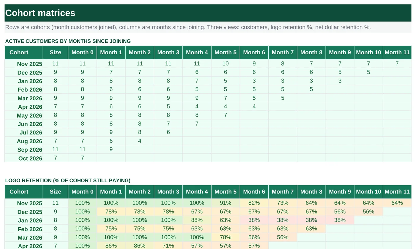
The triangle chart every SaaS board deck has, built from two simple lists. Type one row per customer (cohort month, churn month, MRR) and one row per customer per month in the MRR log; the Cohorts tab counts who is still paying and what they pay, by cohort and by months since they joined, and colors the result. Filled in with 102 fictional customers across 12 cohorts.
- Sheets:
- 5
- Works with:
- Excel for Microsoft 365, Excel 2016 or later, Excel for Mac and Excel for the web
- Updated:
What you can do with it
- See what share of each monthly cohort is still paying 1, 3, 6 and 11 months later
- See net dollar retention, which includes expansion and downgrades, not just churn
- Compare cohorts with a heat map and per-month averages
- Keep raw data in two flat lists that any billing export can fill
What's inside
The workbook has 5 sheets. You only type on a few of them; the rest calculate.
| Sheet | What it's for | You enter | Calculated for you |
|---|---|---|---|
| Start Here | Settings and headline retention numbers | First cohort month, latest month with data | Customers acquired and active, latest MRR, average month-3 and month-6 retention, month-6 NDR, best cohort |
| Customers | One row per customer (room for 150) | Customer, cohort month, churn month (blank while active), starting MRR | Status, months active |
| MRR Log | One row per customer per month (room for 1,000) | Month, customer, MRR | Cohort, looked up from Customers |
| Cohorts | Three matrices: active customers, logo retention %, net dollar retention % | Nothing | Every cell, plus cohort sizes and per-month averages |
| Checks | Five data checks | Nothing | OK or Review |
Before you start
- Export two things from billing: a customer list with first and last paid month, and a monthly MRR history. Dates must be the first of the month.
- Decide what counts as churn. The template treats a customer as churned from the month in the churn column onward; a customer who comes back should be a new row with a new cohort.
- The matrix covers 12 cohorts and 12 months of age. Older or longer histories work if you extend the ranges (see tips).
Step-by-step guide
Set the two dates on Start Here
B6 is the first cohort month shown in the matrices; B7 is the latest month you have data for. Cells for months after B7 stay blank instead of showing a misleading 0.
Fill the Customers tab
One row per customer: name, cohort month (first paid month, as the 1st of the month), churn month (leave blank while the customer is active) and starting MRR. Status and months active calculate.
Fill the MRR Log tab
One row per customer per month with the MRR billed that month. The cohort column looks each customer up on the Customers tab and shows "Not found" if a name is misspelled.
Read the Cohorts tab
Three blocks. The first counts active customers; the second divides by the cohort size to give logo retention %; the third divides each month's MRR by the cohort's month-0 MRR to give net dollar retention %. Rows are cohorts, columns are months since joining, so each row reads left to right as that cohort ages.
Compare cohorts
The heat map colors cells from red (30%) through amber (80%) to green (110%). The Average row at the bottom of each block is the typical curve; a cohort row that is greener than the average row is doing better than usual.
Check the Checks tab
Catches MRR log names that are not on the Customers tab, duplicate customer names, churn months before cohort months, dates that are not the 1st, and a latest month earlier than the first cohort.
Formula map
Every formula in the workbook, grouped by the sheet and column it lives in. A column of copied formulas counts once; the range it covers is shown.
| Sheet | Cells | Functions | What it computes | Reads | Feeds |
|---|---|---|---|---|---|
| Customers | F5 copied down to row 154 | IF, YEAR, MONTH | Months active | B5, C5 | A quick lifetime figure per customer; the matrices do not depend on it. |
| MRR Log | D5 copied down to row 1004 | IF, IFERROR, INDEX, MATCH | Cohort lookup | B5 | The NDR block sums MRR where this column equals the cohort. |
| Cohorts | A7 copied down to row 49 | DATE, YEAR, MONTH | Cohort month sequence | A6 | Every COUNTIFS and SUMIFS in the row uses this as the cohort key. |
| Cohorts | B6 copied down to row 49 | COUNTIF | Cohort size | — | The denominator of logo retention %. |
| Cohorts | C6 copied down to row 17 | IF, DATE, YEAR, MONTH, COUNTIFS | Active customers at a given age | — | The logo retention block divides these counts by the cohort size. |
| Cohorts | C22 filled from C22 to N33 | IF, OR | Logo retention % | — | Start Here averages column F (month 3) and I (month 6) of this block. |
| Cohorts | C38 copied down to row 49 | IF, DATE, YEAR, MONTH, SUMIFS | Net dollar retention % | — | Start Here B14 averages month 6 of this block. |
| Cohorts | C34 filled from C34 to N50 | IFERROR, AVERAGE | Per-month average | — | The typical retention curve to compare each cohort against. |
| Start Here | B10 | COUNTIFS | Customers active now | — | Shown with the total ever acquired in B9. |
| Start Here | B15 | IFERROR, INDEX, MATCH, MAX | Best cohort by month-3 retention | — | Worth asking what that cohort had in common: channel, pricing, onboarding. |
| Checks | B6 | IF, SUMPRODUCT, COUNTIF | No duplicate customer names | — | Duplicates double-count in every matrix. |
Every formula, explained
Each formula below is copied straight from the file, so what you read here is exactly what the cell contains. Click any cell in Excel to see it in the formula bar.
=IF(A5="", "", IF(C5="", (YEAR('Start Here'!$B$7)-YEAR(B5))*12+MONTH('Start Here'!$B$7)-MONTH(B5)+1,
    (YEAR(C5)-YEAR(B5))*12+MONTH(C5)-MONTH(B5)))
Months from the cohort month to the churn month, or to the latest data month plus one for active customers. The year-and-month arithmetic avoids depending on day counts.
Piece by piece
C5=""- Still active: count up to the latest month (Start Here B7) inclusive, hence the +1.
(YEAR(C5)-YEAR(B5))*12+MONTH(C5)-MONTH(B5)- Whole months between two first-of-month dates.
With the sample data: B5 = Nov 1, 2025, C5 = — → F5 result 12
How it is used: A quick lifetime figure per customer; the matrices do not depend on it.
How to change it: Nothing to change.
Learn this: Text and Date Functions in Excel →=IF(B5="", "", IFERROR(INDEX(Customers!$B$5:$B$154, MATCH(B5, Customers!$A$5:$A$154, 0)),
"Not found"))Finds the customer on the Customers tab and returns their cohort month, so the revenue matrix can group MRR rows by cohort.
Piece by piece
MATCH(B5, Customers!$A$5:$A$154, 0)- Row position of the customer name (exact match).
INDEX(Customers!$B$5:$B$154, …)- The cohort month in that row.
IFERROR(…, "Not found")- A misspelled name shows "Not found" instead of #N/A, and the Checks tab counts those.
With the sample data: B5 = Birch Labs 001 → D5 result Nov 1, 2025
How it is used: The NDR block sums MRR where this column equals the cohort.
How to change it: Nothing to change.
Learn this: How to Use INDEX and MATCH in Excel →=DATE(YEAR(A6), MONTH(A6)+1, 1)Each row is the month after the previous one. The first row links to Start Here B6.
Piece by piece
DATE(YEAR(A6), MONTH(A6)+1, 1)- DATE rolls MONTH()+1 over into the next year on its own (month 13 becomes January).
With the sample data: A6 = Nov 1, 2025 → A7 result Dec 1, 2025
How it is used: Every COUNTIFS and SUMIFS in the row uses this as the cohort key.
How to change it: Nothing to change.
Learn this: Text and Date Functions in Excel →=COUNTIF(Customers!$B$5:$B$154, $A6)How many customers joined in this month.
Piece by piece
Customers!$B$5:$B$154- The cohort-month column.
$A6- This row's cohort month.
With the sample data: B6 result 11
How it is used: The denominator of logo retention %.
How to change it: Nothing to change.
Learn this: How to Use COUNTIF and COUNTIFS in Excel →=IF(DATE(YEAR($A6), MONTH($A6)+0,
1)>'Start Here'!$B$7, "",
COUNTIFS(Customers!$B$5:$B$154,
$A6, Customers!$C$5:$C$154,
"")+COUNTIFS(Customers!$B$5:$B$154,
$A6, Customers!$C$5:$C$154,
">"&DATE(YEAR($A6), MONTH($A6)+0, 1)))Customers from the cohort who are still active (no churn month) plus those who churned after the month in question. Columns D to N use the same formula with the offset 1 to 11 in place of 0.
Piece by piece
DATE(YEAR($A6), MONTH($A6)+0, 1)>'Start Here'!$B$7- If this cell's month is after the latest data month, show blank.
COUNTIFS(cohort, $A6, churn, "")- Still active customers in the cohort.
COUNTIFS(cohort, $A6, churn, ">"&DATE(…))- Churned, but after this month, so they were still paying then.
With the sample data: C6 result 11
How it is used: The logo retention block divides these counts by the cohort size.
How to change it: To extend beyond 11 months, copy column N to the right and change the offset in the copied formula to 12, 13, …
Learn this: How to Use COUNTIF and COUNTIFS in Excel →=IF(OR(C6="", $B22=0), "", C6/$B22)Active customers at that age divided by the cohort size. Blank where the count is blank or the cohort is empty.
Piece by piece
C6=""- No data for that month yet: stay blank.
$B22=0- Empty cohort: stay blank rather than divide by zero.
C6/$B22- Active ÷ size. $B keeps the size column fixed when copying across.
With the sample data: C22 result 1
How it is used: Start Here averages column F (month 3) and I (month 6) of this block.
How to change it: Nothing to change.
Learn this: Relative, Absolute and Mixed References in Excel →=IF(DATE(YEAR($A38), MONTH($A38)+0,
1)>'Start Here'!$B$7, "",
IF(SUMIFS('MRR Log'!$C$5:$C$1004, 'MRR Log'!$D$5:$D$1004, $A38, 'MRR Log'!$A$5:$A$1004, $A38)=0,
"", SUMIFS('MRR Log'!$C$5:$C$1004, 'MRR Log'!$D$5:$D$1004, $A38, 'MRR Log'!$A$5:$A$1004, DATE(YEAR($A38), MONTH($A38)+0, 1))/SUMIFS('MRR Log'!$C$5:$C$1004, 'MRR Log'!$D$5:$D$1004, $A38, 'MRR Log'!$A$5:$A$1004, $A38)))MRR from the cohort in a given month divided by the cohort's MRR in its first month. Above 100% means expansions outweigh churn and downgrades.
Piece by piece
SUMIFS('MRR Log'!$C$5:$C$1004, 'MRR Log'!$D$5:$D$1004, $A38, 'MRR Log'!$A$5:$A$1004, DATE(…))- MRR in the target month from customers whose looked-up cohort equals this row.
SUMIFS(…, $A38)- The same sum for the cohort's own month (month 0).
IF(…=0, "", …)- Blank if the cohort has no month-0 revenue.
With the sample data: C38 result 1
How it is used: Start Here B14 averages month 6 of this block.
How to change it: Nothing to change.
Learn this: How to Use SUMIF and SUMIFS in Excel →=IFERROR(AVERAGE(C22:C33), "")The average of the twelve cohort rows for one age column, ignoring blanks. IFERROR covers the case where a whole column is blank.
Piece by piece
AVERAGE(C22:C33)- AVERAGE skips blank cells automatically.
IFERROR(…, "")- When there is nothing to average.
With the sample data: C34 result 1
How it is used: The typical retention curve to compare each cohort against.
How to change it: Nothing to change.
Learn this: How to Use the AVERAGE Function in Excel →=COUNTIFS(Customers!$A$5:$A$154,
"<>", Customers!$C$5:$C$154,
"")Counts customers with a name but no churn month.
Piece by piece
Customers!$A$5:$A$154, "<>"- Has a name.
Customers!$C$5:$C$154, ""- Churn month is blank.
With the sample data: B10 result 69
How it is used: Shown with the total ever acquired in B9.
How to change it: Nothing to change.
Learn this: How to Use COUNTIF and COUNTIFS in Excel →=IFERROR(INDEX(Cohorts!$A$22:$A$33,
MATCH(MAX(Cohorts!$F$22:$F$33), Cohorts!$F$22:$F$33, 0)),
"")Finds the highest month-3 logo retention and returns that row's cohort month.
Piece by piece
MAX(Cohorts!$F$22:$F$33)- Highest month-3 retention.
MATCH(…, Cohorts!$F$22:$F$33, 0)- Its row.
INDEX(Cohorts!$A$22:$A$33, …)- The cohort month in that row.
With the sample data: B15 result Nov 1, 2025
How it is used: Worth asking what that cohort had in common: channel, pricing, onboarding.
How to change it: Change F to I in all three references for month 6.
Learn this: How to Use INDEX and MATCH in Excel →=IF(SUMPRODUCT((Customers!$A$5:$A$154<>"")*(COUNTIF(Customers!$A$5:$A$154, Customers!$A$5:$A$154)>1))=0,
"OK", "Review")For every non-blank name, counts how many times it appears; any count above 1 is a duplicate.
Piece by piece
Customers!$A$5:$A$154<>""- Only rows with a name.
COUNTIF(range, range)>1- Counts each name against the whole column; TRUE where a name repeats.
SUMPRODUCT(…)- Adds up the duplicate rows.
With the sample data: B6 result OK
How it is used: Duplicates double-count in every matrix.
How to change it: Nothing to change.
Learn this: How to Use COUNTIF and COUNTIFS in Excel →Tips and limits
- Capacity: 150 customers, 1,000 MRR log rows, 12 cohorts × 12 months. To extend the lists, use Ctrl+H on formulas to replace $154 and $1004 with larger rows; to extend the matrix, copy the last column to the right and adjust the month offset.
- Logo retention answers "how many stayed"; net dollar retention answers "how much revenue stayed". Both are shown because a cohort can lose customers and still grow revenue.
- Customers who leave and return later should be entered as a new customer row (append -2 to the name) so both cohorts stay honest.
- For a single blended churn rate and LTV, see the SaaS Unit Economics template on this site.
Learn the skills behind this template
Was this guide helpful? Spot a mistake? Send feedback · admin@arumsoft.com