Restaurant Prime Cost Calculator for Excel
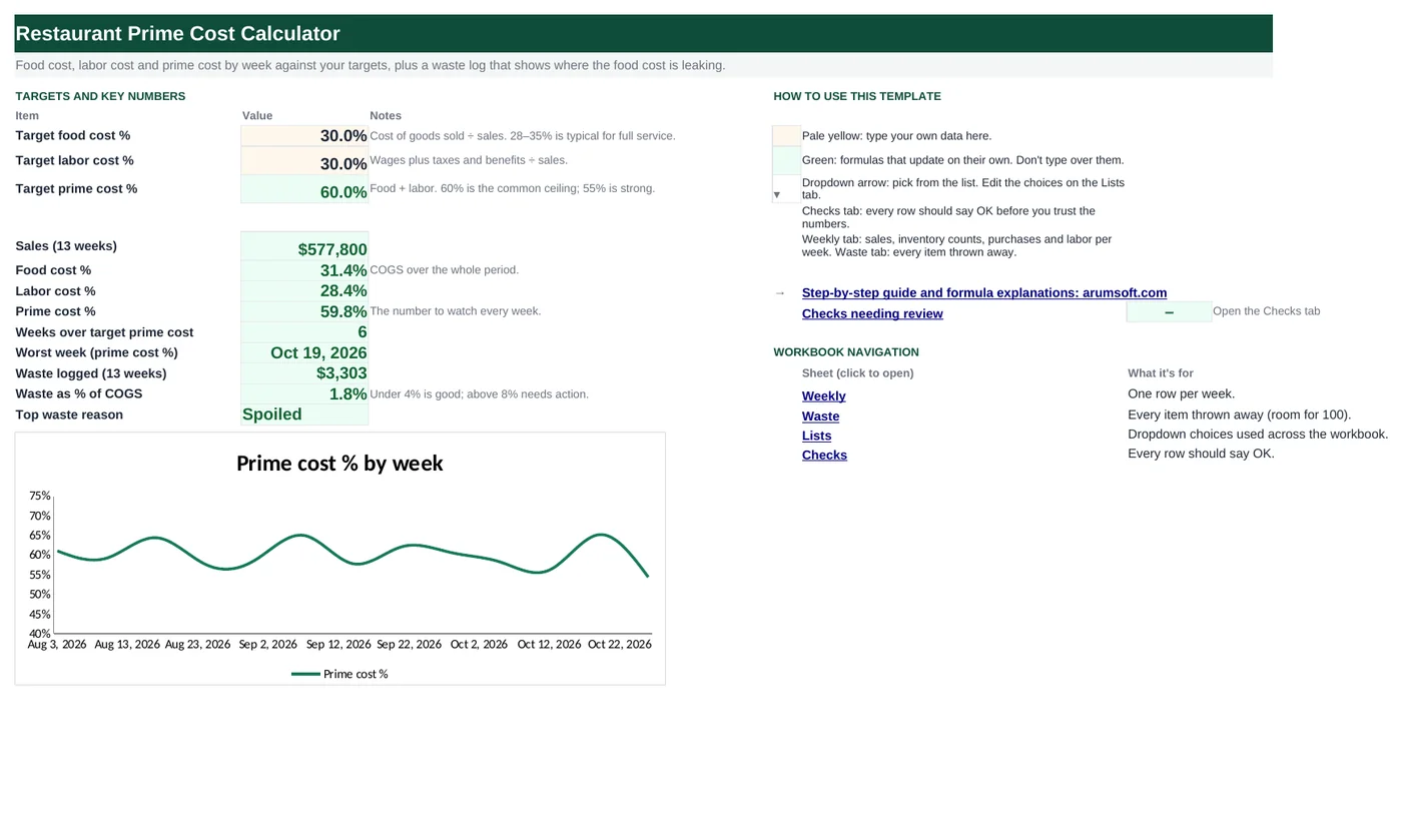
Prime cost is food plus labor as a share of sales, and it is the one number that decides whether a restaurant makes money. This workbook takes a weekly inventory count, purchases, sales and payroll, works out COGS and prime cost for every week, flags the weeks that miss your target, and keeps a waste log so you can see which part of the food cost is going in the bin.
- Sheets:
- 5
- Works with:
- Excel for Microsoft 365, Excel 2016 or later, Excel for Mac and Excel for the web
- Updated:
What you can do with it
- Weekly food cost %, labor % and prime cost % against the targets you set
- COGS from beginning inventory + purchases − ending inventory, with the count carried forward automatically
- A waste log with cost by reason and waste as a share of COGS
- A 13-week prime cost chart and six data checks
What's inside
The workbook has 5 sheets. You only type on a few of them; the rest calculate.
| Sheet | What it's for | You enter | Calculated for you |
|---|---|---|---|
| Start Here | Targets and the 13-week summary | Target food cost % and labor % | Prime cost target, period sales, food cost %, labor %, prime cost %, weeks over target, worst week, waste total and share, top waste reason |
| Weekly | One row per week (13) | Food and beverage sales, beginning inventory (first week only), purchases, ending inventory, wages, taxes and benefits | Total sales, COGS, food cost %, labor cost, labor %, prime cost %, gap to target, status |
| Waste | Every item thrown away (room for 100) | Date, item, category, quantity, unit, unit cost, reason | Cost, week starting, cost by reason with share |
| Lists | Dropdowns | Categories, reasons, units | Nothing |
| Checks | Six data checks | Nothing | OK or Review |
Before you start
- Decide your targets. Full-service restaurants usually aim for food cost around 28–35% and labor around 25–35%, for a prime cost at or under 60%.
- Pick one day a week for the inventory count and stick to it; the workbook assumes weeks start on Monday.
- Have weekly sales from the POS and weekly payroll (gross wages plus employer taxes and benefits) to hand.
Step-by-step guide
Set the targets
Start Here B6 and B7. B8 adds them to give the prime cost target that every week is compared against.
Enter the first week's beginning inventory
Weekly E5 is the only beginning inventory you type. Every later week links to the previous week's ending count, so one count per week is enough.
Fill in each week
Food sales, beverage sales, purchases, ending inventory, wages, and taxes and benefits. COGS, the percentages and the status calculate. "Close" means within 3 points over target; "Over" means more than that.
Log waste as it happens
Waste tab: date, item, category, quantity, unit, unit cost and a reason from the dropdown. Cost and the week it belongs to calculate, and the summary on the right totals by reason.
Read Start Here
Period food cost %, labor % and prime cost %; how many weeks missed the target and which was worst; waste as a share of COGS (under 4% is good) and the reason that costs most.
Check the Checks tab
It catches weeks that are not consecutive Mondays, an ending inventory larger than beginning plus purchases, negative counts, waste dated outside the period, waste rows without a reason, and a prime cost target above 70%.
Formula map
Every formula in the workbook, grouped by the sheet and column it lives in. A column of copied formulas counts once; the range it covers is shown.
| Sheet | Cells | Functions | What it computes | Reads | Feeds |
|---|---|---|---|---|---|
| Weekly | E6 copied down to row 17 | arithmetic | Beginning inventory carried forward | G5 | Feeds COGS in column H. |
| Weekly | H5 copied down to row 17 | arithmetic | Cost of goods sold | E5, F5, G5 | Food cost % divides this by total sales; Start Here B11 sums the column for the period. |
| Weekly | I5 copied down to row 18 | IF | Food cost % | H5, D5 | Added to labor % to give prime cost %. |
| Weekly | N5 copied down to row 18 | IF | Prime cost % | I5, M5 | Compared with the target in column O and P; charted on Start Here. |
| Weekly | P5 copied down to row 17 | IF | Status | N5 | Conditional formatting colors the three states. |
| Start Here | B14 | COUNTIF | Weeks over target | B8 | A quick read on how consistent the period was. |
| Start Here | B15 | IFERROR, INDEX, MATCH, MAX | Worst week | — | Tells you where to start looking. |
| Waste | I5 copied down to row 104 | IF, WEEKDAY | Week starting | A5 | Lets you compare waste with the Weekly tab week by week (a pivot or SUMIF on this column). |
| Waste | L5 copied down to row 11 | IF, SUMIF | Cost by reason | — | M5 divides by the total for the share; Start Here B18 names the biggest reason. |
| Start Here | B17 | IF, SUM | Waste as % of COGS | B16 | Under 4% is good; above 8% needs action. |
| Checks | B5 | IF, AND, WEEKDAY, SUMPRODUCT | Weeks are consecutive Mondays | — | A missed or duplicated week would distort the carried-forward inventory. |
Every formula, explained
Each formula below is copied straight from the file, so what you read here is exactly what the cell contains. Click any cell in Excel to see it in the formula bar.
=G5Each week starts with what the previous week ended with. Only the first week (E5) is typed.
Piece by piece
G5- Previous week's ending inventory.
With the sample data: G5 = 10,192 → E6 result 10,192
How it is used: Feeds COGS in column H.
How to change it: If you re-count at the start of a week and the number differs, type over the link for that week only.
Learn this: How to Write Basic Formulas in Excel →=E5+F5-G5What you used this week: what you had, plus what you bought, minus what is left.
Piece by piece
E5- Beginning inventory.
+F5- Purchases received this week.
-G5- Ending inventory count.
With the sample data: E5 = 9,800, F5 = 12,534, G5 = 10,192 → H5 result 12,142
How it is used: Food cost % divides this by total sales; Start Here B11 sums the column for the period.
How to change it: Nothing to change.
Learn this: How to Write Basic Formulas in Excel →=IF(D5=0, "", H5/D5)COGS divided by total sales, blank when there are no sales yet so an empty week does not show a divide-by-zero error.
Piece by piece
D5=0- No sales: show nothing.
H5/D5- COGS ÷ total sales.
With the sample data: H5 = 12,142, D5 = 40,600 → I5 result 29.9%
How it is used: Added to labor % to give prime cost %.
How to change it: To measure food cost against food sales only (excluding beverages), divide by B5 instead of D5.
Learn this: How to Use the IF Function in Excel →=IF(D5=0, "", I5+M5)Food cost % plus labor %. The key number.
Piece by piece
D5=0- No sales: show nothing.
I5+M5- Food cost % + labor %.
With the sample data: I5 = 29.9%, M5 = 31.1% → N5 result 61.0%
How it is used: Compared with the target in column O and P; charted on Start Here.
How to change it: Nothing to change.
Learn this: How to Write Basic Formulas in Excel →=IF(N5="", "", IF(N5<='Start Here'!$B$8,
"On target", IF(N5<='Start Here'!$B$8+0.03, "Close", "Over")))On target when prime cost is at or under the target; Close when it is within three points over; Over beyond that.
Piece by piece
N5=""- No data: show nothing.
N5<='Start Here'!$B$8- At or under target.
N5<='Start Here'!$B$8+0.03- Within 3 points over.
With the sample data: N5 = 61.0% → P5 result Close
How it is used: Conditional formatting colors the three states.
How to change it: Change 0.03 to widen or narrow the Close band.
Learn this: How to Use the IF Function in Excel →=COUNTIF(Weekly!$N$5:$N$17, ">"&B8)Counts weeks whose prime cost % is above the target. The comparison is built as text: ">" joined to the target value.
Piece by piece
Weekly!$N$5:$N$17- Prime cost % for every week.
">"&B8- The criterion: greater than the target.
With the sample data: B8 = 60.0% → B14 result 6
How it is used: A quick read on how consistent the period was.
How to change it: Nothing to change.
Learn this: How to Use COUNTIF and COUNTIFS in Excel →=IFERROR(INDEX(Weekly!$A$5:$A$17,
MATCH(MAX(Weekly!$N$5:$N$17), Weekly!$N$5:$N$17, 0)),
"")Finds the highest prime cost % and returns the week-starting date on that row.
Piece by piece
MAX(Weekly!$N$5:$N$17)- The highest prime cost %.
MATCH(…, Weekly!$N$5:$N$17, 0)- Which row it is on.
INDEX(Weekly!$A$5:$A$17, …)- The date on that row.
IFERROR(…, "")- Blank until there is data.
With the sample data: B15 result Oct 19, 2026
How it is used: Tells you where to start looking.
How to change it: Nothing to change.
Learn this: How to Use INDEX and MATCH in Excel →=IF(A5="", "", A5-WEEKDAY(A5, 2)+1)Converts any date to the Monday of its week. WEEKDAY with return type 2 gives Monday = 1 … Sunday = 7, so subtracting it and adding 1 lands on Monday.
Piece by piece
A5- The waste date.
WEEKDAY(A5, 2)- 1 for Monday through 7 for Sunday.
A5-…+1- Back to Monday.
With the sample data: A5 = Aug 3, 2026 → I5 result Aug 3, 2026
How it is used: Lets you compare waste with the Weekly tab week by week (a pivot or SUMIF on this column).
How to change it: For weeks starting Sunday, use A5-WEEKDAY(A5,1)+1.
Learn this: Text and Date Functions in Excel →=IF(K5="", "", SUMIF($G$5:$G$104, K5, $H$5:$H$104))Adds the cost of every waste row whose reason matches the label in column K, which is pulled from the Lists tab.
Piece by piece
$G$5:$G$104- Reason column.
K5- The reason to match.
$H$5:$H$104- Costs to add.
With the sample data: L5 result 1,506.2
How it is used: M5 divides by the total for the share; Start Here B18 names the biggest reason.
How to change it: Nothing to change; add reasons on the Lists tab.
Learn this: How to Use SUMIF and SUMIFS in Excel →=IF(SUM(Weekly!$H$5:$H$17)=0, 0, B16/SUM(Weekly!$H$5:$H$17))Total logged waste divided by total COGS for the period.
Piece by piece
SUM(Weekly!$H$5:$H$17)=0- No COGS yet: show 0.
B16/SUM(Weekly!$H$5:$H$17)- Waste ÷ COGS.
With the sample data: B16 = 3,302.5 → B17 result 1.8%
How it is used: Under 4% is good; above 8% needs action.
How to change it: Nothing to change.
Learn this: How to Use the IF Function in Excel →=IF(AND(WEEKDAY(Weekly!$A$5, 2)=1,
SUMPRODUCT(--(Weekly!$A$6:$A$17-Weekly!$A$5:$A$16<>7))=0),
"OK", "Review")Checks that the first date is a Monday and that every later date is exactly 7 days after the one before.
Piece by piece
WEEKDAY(Weekly!$A$5, 2)=1- First week starts on a Monday.
Weekly!$A$6:$A$17-Weekly!$A$5:$A$16<>7- TRUE for any gap that is not 7 days.
SUMPRODUCT(--(…))=0- No such gaps.
With the sample data: B5 result OK
How it is used: A missed or duplicated week would distort the carried-forward inventory.
How to change it: Nothing to change.
Learn this: How to Use SUMIF and SUMIFS in Excel →Tips and limits
- Capacity: 13 weeks on the Weekly tab, 100 waste rows. For a new quarter, save a copy, type the new first-week beginning inventory in E5 (last quarter's final count), and clear the rest.
- Count inventory at the same time every week, before deliveries. A count taken after a delivery inflates ending inventory and understates COGS.
- Include employer payroll taxes and benefits in labor, not just wages; leaving them out understates prime cost by several points.
- The chart on Start Here plots prime cost % by week. Add a second series pointing at Start Here B8 if you want the target drawn as a line.
- Waste as a share of COGS is only as good as the log. Make it a closing task for the kitchen lead, not an afterthought.
Learn the skills behind this template
Was this guide helpful? Spot a mistake? Send feedback · admin@arumsoft.com