FMEA Risk Priority Number Matrix for Excel
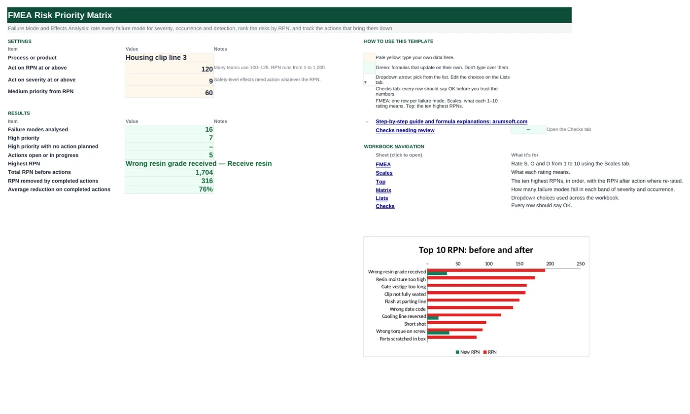
A Failure Mode and Effects Analysis asks three questions about everything that can go wrong in a process: how bad is it (severity), how often does it happen (occurrence), and how likely is your current control to catch it (detection). Multiply the three 1–10 ratings and you have the Risk Priority Number. This workbook calculates the RPN, sets a priority that also catches any safety-level severity, ranks the risks, tracks the actions that reduce them, and measures how much each action took off.
- Sheets:
- 7
- Works with:
- Excel for Microsoft 365, Excel 2016 or later, Excel for Mac and Excel for the web
- Updated:
What you can do with it
- RPN = S × O × D for up to 50 failure modes, with a color scale and S × O criticality
- Priority High / Medium / Low from an RPN threshold plus an always-act severity level
- Recommended action, owner, due date and status, re-rated S, O and D, new RPN and % reduction
- Top 10 risks before and after, a severity × occurrence matrix, and flags for missing or overdue actions
What's inside
The workbook has 7 sheets. You only type on a few of them; the rest calculate.
| Sheet | What it's for | You enter | Calculated for you |
|---|---|---|---|
| Start Here | Thresholds and the summary | Process name, RPN action threshold, always-act severity, medium threshold | Failure modes, high priority, high with no action, actions open, highest RPN, total RPN, RPN removed, average reduction |
| FMEA | The worksheet (50 rows) | Step, failure mode, effect, S, cause, O, controls, D, action, owner, due, status, new S, O, D | RPN, S × O, priority, rank, new RPN, reduction, flag |
| Scales | Meaning of 1–10 | Wording for each rating | Nothing |
| Top | Ten highest RPNs | Nothing | Failure mode, step, RPN, priority, new RPN, status in rank order |
| Matrix | Severity × occurrence bands | Band limits | Count of failure modes per cell |
| Lists | Action status | Status choices | Nothing |
| Checks | Six data checks | Nothing | OK or Review |
Before you start
- Map the process steps first (a flowchart or the routing).
- Agree the rating scales with the team before scoring; adapt the Scales tab wording to your product.
- Score as a team. One person's FMEA misses failure modes.
Step-by-step guide
Set the thresholds
Start Here B7–B9: the RPN that needs action, the severity that always needs action (9 or 10 usually means safety), and where Medium starts.
List the failure modes
FMEA tab columns B–D: for each process step, how it can fail and what the customer or next step would see.
Rate S, O and D
Columns E, G, I with the causes and current controls in F and H. RPN, priority and rank calculate.
Plan actions
For High rows, enter an action, owner and due date in N–P. The flag column says Needs action until you do.
Re-rate after action
When an action is Done, enter the new S, O and D in R–T. New RPN and the reduction appear.
Review
Top tab and the Start Here chart show the ten worst risks before and after; the Matrix tab shows where risk concentrates.
Formula map
Every formula in the workbook, grouped by the sheet and column it lives in. A column of copied formulas counts once; the range it covers is shown.
| Sheet | Cells | Functions | What it computes | Reads | Feeds |
|---|---|---|---|---|---|
| FMEA | J6 copied down to row 55 | IF, COUNT | Risk Priority Number | E6, G6, I6 | Priority, rank, the Top tab and the chart all use it. |
| FMEA | L6 copied down to row 55 | IF, OR | Priority | J6, E6 | Colored and counted on Start Here B14. |
| FMEA | M6 copied down to row 55 | IF, RANK, COUNTIF | Unique rank | J6 | The Top tab looks ranks 1–10 up. |
| FMEA | V6 copied down to row 55 | IF, OR | Reduction after action | U6, J6 | Averaged on Start Here B20. |
| FMEA | W6 copied down to row 55 | IF, AND, TODAY | Action flag | L6, N6, Q6, P6 | Filter the column to run the review meeting. |
| Top | B5 copied down to row 14 | IFERROR, MATCH | Row of rank 1 | A5 | Columns C–H use INDEX with this position to pull the failure mode, step, RPN and status. |
| Matrix | B6 copied down to row 10 | COUNTIFS | Failure modes in a band | — | Color shows the risk zone: top right is worst. |
| Start Here | B19 | SUMPRODUCT, IFERROR | RPN removed by completed actions | — | The headline result of the FMEA effort. |
Every formula, explained
Each formula below is copied straight from the file, so what you read here is exactly what the cell contains. Click any cell in Excel to see it in the formula bar.
=IF(COUNT(E6, G6, I6)<3, "", E6*G6*I6)Severity × occurrence × detection, only when all three ratings are entered.
Piece by piece
COUNT(E6, G6, I6)<3- Any rating missing: blank.
E6*G6*I6- The RPN, from 1 to 1,000.
With the sample data: E6 = 8, G6 = 4, I6 = 6 → J6 result 192
How it is used: Priority, rank, the Top tab and the chart all use it.
How to change it: Nothing to change.
Learn this: How to Write Basic Formulas in Excel →=IF(J6="", "", IF(OR(J6>='Start Here'!$B$7, E6>='Start Here'!$B$8),
"High", IF(J6>='Start Here'!$B$9, "Medium", "Low")))High if the RPN reaches the action threshold or severity reaches the always-act level; Medium from the medium threshold; Low otherwise.
Piece by piece
OR(J6>='Start Here'!$B$7, E6>='Start Here'!$B$8)- High: RPN ≥ 120 or S ≥ 9.
J6>='Start Here'!$B$9- Medium: RPN ≥ 60.
With the sample data: J6 = 192, E6 = 8 → L6 result High
How it is used: Colored and counted on Start Here B14.
How to change it: Change the thresholds on Start Here.
Learn this: How to Use AND and OR in Excel →=IF(J6="", "", RANK(J6, $J$6:$J$55, 0)+COUNTIF($J$6:J6, J6)-1)Ranks the RPN from highest down and breaks ties by order on the sheet.
Piece by piece
RANK(J6, $J$6:$J$55, 0)- 1 = highest RPN.
+COUNTIF($J$6:J6, J6)-1- Second of two equal RPNs gets the next rank.
With the sample data: J6 = 192 → M6 result 1
How it is used: The Top tab looks ranks 1–10 up.
How to change it: Nothing to change.
Learn this: How to Use COUNTIF and COUNTIFS in Excel →=IF(OR(U6="", J6=""), "", 1-U6/J6)One minus new RPN ÷ original RPN.
Piece by piece
U6- New RPN = new S × new O × new D.
1-U6/J6- Share of the risk removed.
With the sample data: U6 = 32, J6 = 192 → V6 result 83.3%
How it is used: Averaged on Start Here B20.
How to change it: Nothing to change.
Learn this: How to Write Basic Formulas in Excel →=IF(J6="", "", IF(AND(L6="High", N6=""),
"Needs action", IF(AND(Q6<>"Done", P6<>"", P6<TODAY()), "Overdue", IF(AND(Q6="Done", U6=""), "Re-rate", IF(AND(U6<>"", U6>='Start Here'!$B$7), "Still high", "")))))Points at what needs attention: a High row with no action, an action past its due date, a Done action not yet re-rated, or a new RPN still above the threshold.
Piece by piece
AND(L6="High", N6="")- "Needs action".
AND(Q6<>"Done", P6<TODAY())- "Overdue".
AND(Q6="Done", U6="")- "Re-rate".
U6>='Start Here'!$B$7- "Still high".
With the sample data: L6 = High, N6 = Barcode scan against PO at receiving, Q6 = Done, P6 = Oct 15, 2026 → W6 result —
How it is used: Filter the column to run the review meeting.
How to change it: Nothing to change.
Learn this: How to Use TODAY and NOW in Excel →=IFERROR(MATCH(A5, FMEA!$M$6:$M$55, 0), "")Finds which FMEA row holds rank 1 (2, 3 … in the rows below).
Piece by piece
MATCH(A5, FMEA!$M$6:$M$55, 0)- Position of this rank.
IFERROR(…, "")- Blank when fewer rows exist.
With the sample data: A5 = 1 → B5 result 1
How it is used: Columns C–H use INDEX with this position to pull the failure mode, step, RPN and status.
How to change it: Nothing to change.
Learn this: How to Use INDEX and MATCH in Excel →=COUNTIFS(FMEA!$E$6:$E$55,
">="&$H6, FMEA!$E$6:$E$55,
"<="&$I6, FMEA!$G$6:$G$55,
">="&B$12, FMEA!$G$6:$G$55,
"<="&B$13)Counts failure modes whose severity and occurrence both fall inside this cell's bands.
Piece by piece
FMEA!$E$6:$E$55, ">="&$H6, …, "<="&$I6- Severity in the row band (9–10 here).
FMEA!$G$6:$G$55, ">="&B$12, …, "<="&B$13- Occurrence in the column band.
With the sample data: B6 result 0
How it is used: Color shows the risk zone: top right is worst.
How to change it: Change the band limits in H:I and rows 12–13.
Learn this: How to Use COUNTIF and COUNTIFS in Excel →=SUMPRODUCT(IFERROR((FMEA!$U$6:$U$55<>"")*(FMEA!$J$6:$J$55-FMEA!$U$6:$U$55),
0))For every row that has been re-rated, original RPN minus new RPN, added up.
Piece by piece
(FMEA!$U$6:$U$55<>"")- 1 for re-rated rows.
*(FMEA!$J$6:$J$55-FMEA!$U$6:$U$55)- Times the drop in RPN.
IFERROR(…, 0)- Blank rows give 0.
With the sample data: B19 result 316
How it is used: The headline result of the FMEA effort.
How to change it: Nothing to change.
Learn this: How to Use IFERROR in Excel →Tips and limits
- Capacity: 50 failure modes. Insert rows inside the table to add more; the ranges stretch.
- RPN alone can mislead: 10 × 2 × 2 = 40 is a safety issue, 4 × 5 × 5 = 100 is not. That is why severity has its own threshold.
- Newer FMEA handbooks (AIAG-VDA, 2019) rank by Action Priority tables instead of RPN; this workbook uses the classic RPN, which most teams still recognize.
- Detection is rated on the current control, not on a control you plan to add. Re-rate after it is in place.
- Keep the FMEA alive: review it after any customer complaint, process change or new failure.
Learn the skills behind this template
Was this guide helpful? Spot a mistake? Send feedback · admin@arumsoft.com