Short-Term Rental Occupancy and Net Yield Tracker for Excel
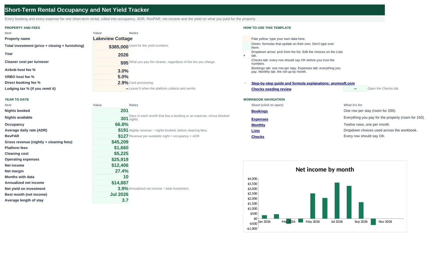
Platform dashboards show gross bookings; they do not show what you keep. This workbook logs every stay with its platform, nightly rate and cleaning fee, applies the host fee for that platform, counts your cleaner's cost per turnover, logs every expense, and rolls it all up by month into occupancy, average daily rate, RevPAR and net income. The Start Here sheet annualizes the result into a net yield on what you paid for the property.
- Sheets:
- 6
- Works with:
- Excel for Microsoft 365, Excel 2016 or later, Excel for Mac and Excel for the web
- Updated:
Short-Term Rental Occupancy and Net Yield Tracker.xlsx
Free to download. No sign-up needed.
What you can do with it
- Booking log with per-platform host fees and payouts
- Monthly occupancy, ADR, RevPAR and net income, with blocked nights excluded
- Expense log with year-to-date totals by category
- Annualized net income and net yield on your total investment
What's inside
The workbook has 6 sheets. You only type on a few of them; the rest calculate.
| Sheet | What it's for | You enter | Calculated for you |
|---|---|---|---|
| Start Here | Settings and the year-to-date summary | Property, total investment, year, cleaner cost, host fee % per platform, lodging tax | Nights booked and available, occupancy, ADR, RevPAR, revenue, fees, cleaning, expenses, net income and margin, annualized income, net yield, best month, average stay |
| Bookings | One row per stay (200) | Check-in, nights, platform, guest, guests, nightly rate, cleaning fee charged, status | Check-out, nightly revenue, gross, platform fee, payout, month |
| Expenses | Everything you pay (150) | Date, category, vendor, amount | Month, year-to-date by category |
| Monthly | Twelve rows | Blocked nights | Nights available and booked, revenue, fees, cleaning cost, expenses, net income, occupancy, ADR, RevPAR |
| Lists | Dropdowns | Platforms, statuses, categories | Nothing |
| Checks | Six data checks | Nothing | OK or Review |
Before you start
- Export your reservations from each platform; you need check-in date, nights, nightly rate and the cleaning fee charged.
- Know each platform's host fee: the simplified Airbnb host-only fee is about 3% (15% under the host-only model), VRBO 5% plus payment processing, direct bookings whatever your card processor charges.
- Decide the total investment you want the yield measured against: purchase price plus closing costs plus furnishing.
Step-by-step guide
Set the property and fees
Start Here B6–B13: name, total investment, year, what you pay the cleaner per turnover, host fee % by platform, lodging tax if you remit it yourself.
Log bookings
Bookings tab: check-in, nights, platform, guest, nightly rate, cleaning fee charged, status. Check-out, revenue, platform fee and payout calculate; a stay belongs to its check-in month.
Log expenses
Expenses tab: date, category (dropdown), vendor, amount. Do not log cleaning you pay per turnover; the Monthly tab calculates it from the number of stays.
Block owner nights
Monthly column N: nights the property was blocked for your own use or repairs. They are removed from nights available so occupancy stays honest.
Read the Monthly tab
Occupancy = nights booked ÷ available; ADR = nightly revenue ÷ nights booked; RevPAR = occupancy × ADR; net income = gross − platform fees − cleaning cost − expenses.
Read Start Here
Year-to-date totals, net margin, the annualized net income (net ÷ months with data × 12) and the net yield on your investment. The Checks tab catches overlapping stays, out-of-order rows, missing rates and bookings outside the year.
Formula map
Every formula in the workbook, grouped by the sheet and column it lives in. A column of copied formulas counts once; the range it covers is shown.
| Sheet | Cells | Functions | What it computes | Reads | Feeds |
|---|---|---|---|---|---|
| Bookings | L5 copied down to row 204 | IF | Platform fee | K5, C5 | Payout = gross − fee; the Monthly tab sums fees by month. |
| Bookings | N5 copied down to row 204 | IF, DATE, YEAR, MONTH | Booking month | A5 | Monthly columns C–G match on this. |
| Monthly | B5 copied down to row 16 | IF, OR, DAY, EOMONTH | Nights available | E5, I5, A5, N5 | The denominator for occupancy. |
| Monthly | C5 copied down to row 16 | SUMIFS | Nights booked | A5 | Occupancy and ADR use it. |
| Monthly | H5 copied down to row 16 | arithmetic | Cleaning cost | E5 | Subtracted from gross in net income. The cleaning fee you charge guests is in gross revenue. |
| Monthly | J5 copied down to row 16 | arithmetic | Net income | F5, G5, H5, I5 | Charted on Start Here; summed for the year. |
| Monthly | M5 copied down to row 17 | IF, OR | RevPAR | K5, L5 | Compare month to month and with other listings. |
| Start Here | B29 | IF | Annualized net income | B26, B28 | Net yield divides it by the investment. |
| Start Here | B31 | IFERROR, INDEX, MATCH, MAX | Best month | — | A quick read on seasonality. |
| Checks | B5 | IF, SUMPRODUCT, IFERROR | No overlapping stays | — | A double booking is the costliest data error. |
Every formula, explained
Each formula below is copied straight from the file, so what you read here is exactly what the cell contains. Click any cell in Excel to see it in the formula bar.
=IF(K5="", "", K5*IF(C5="Airbnb",
    'Start Here'!$B$10, IF(C5="VRBO", 'Start Here'!$B$11, 'Start Here'!$B$12)))
Gross (nightly revenue + cleaning fee) times the host fee for the booking's platform, picked with a nested IF.
Piece by piece
K5- Gross for the stay.
C5="Airbnb" → 'Start Here'!$B$10- Airbnb fee.
C5="VRBO" → 'Start Here'!$B$11- VRBO fee.
otherwise 'Start Here'!$B$12- Direct / other.
With the sample data: K5 = 423, C5 = Direct → L5 result 12.27
How it is used: Payout = gross − fee; the Monthly tab sums fees by month.
How to change it: Add another platform by nesting one more IF, or switch to a lookup against the Lists tab.
Learn this: How to Use the IF Function in Excel →=IF(A5="", "", DATE(YEAR(A5), MONTH(A5), 1))The first day of the check-in month, used as the key for every monthly SUMIF.
Piece by piece
YEAR(A5), MONTH(A5)- Year and month of check-in.
DATE(…, 1)- The first of that month.
With the sample data: A5 = Jan 1, 2026 → N5 result Jan 1, 2026
How it is used: Monthly columns C–G match on this.
How to change it: Nothing to change.
Learn this: Text and Date Functions in Excel →=IF(OR(E5>0, I5>0), DAY(EOMONTH(A5, 0))-N5, 0)Days in the month minus blocked nights, but 0 for months with no bookings and no expenses so an empty future month does not count against occupancy.
Piece by piece
OR(E5>0, I5>0)- The month has activity.
DAY(EOMONTH(A5, 0))- Days in the month.
-N5- Blocked nights.
With the sample data: E5 = 5, I5 = 2,875.47, A5 = Jan 1, 2026, N5 = 0 → B5 result 31
How it is used: The denominator for occupancy.
How to change it: To count every month of the year regardless, replace the IF with DAY(EOMONTH(A5,0))-N5.
Learn this: Text and Date Functions in Excel →=SUMIFS(Bookings!$B$5:$B$204,
Bookings!$N$5:$N$204, A5,
Bookings!$H$5:$H$204, "<>Cancelled")Adds nights for stays that check in this month and are not cancelled.
Piece by piece
Bookings!$B$5:$B$204- Nights.
Bookings!$N$5:$N$204, A5- Booking month matches.
Bookings!$H$5:$H$204, "<>Cancelled"- Not cancelled.
With the sample data: A5 = Jan 1, 2026 → C5 result 22
How it is used: Occupancy and ADR use it.
How to change it: Nothing to change.
Learn this: How to Use SUMIF and SUMIFS in Excel →=E5*'Start Here'!$B$9Number of stays times what you pay the cleaner per turnover.
Piece by piece
E5- Stays this month.
'Start Here'!$B$9- Cleaner cost per turnover.
With the sample data: E5 = 5 → H5 result 475
How it is used: Subtracted from gross in net income. The cleaning fee you charge guests is in gross revenue.
How to change it: If cleaning cost varies by stay, add a column on the Bookings tab and SUMIF it instead.
Learn this: Relative, Absolute and Mixed References in Excel →=F5-G5-H5-I5Gross revenue minus platform fees, cleaning cost and expenses.
Piece by piece
F5- Gross (nightly + cleaning fees charged).
-G5- Platform fees.
-H5- Cleaning cost.
-I5- Expenses logged for the month.
With the sample data: F5 = 3,868, G5 = 184.52, H5 = 475, I5 = 2,875.47 → J5 result 333.01
How it is used: Charted on Start Here; summed for the year.
How to change it: Nothing to change.
Learn this: How to Write Basic Formulas in Excel →=IF(OR(B5=0, K5=""), "", K5*L5)Revenue per available night: occupancy times ADR. The one number that combines how often you are booked and at what rate.
Piece by piece
OR(B5=0, K5="")- No available nights: show nothing.
K5*L5- Occupancy × ADR.
With the sample data: K5 = 71.0%, L5 = 147.41 → M5 result 104.61
How it is used: Compare month to month and with other listings.
How to change it: Nothing to change.
Learn this: How to Use the IF Function in Excel →=IF(B28=0, 0, B26/B28*12)Net income so far divided by the months with data, times twelve.
Piece by piece
B28=0- No data: 0.
B26/B28- Average net per month.
*12- A full year.
With the sample data: B26 = 12,405.52, B28 = 10 → B29 result 14,886.63
How it is used: Net yield divides it by the investment.
How to change it: Seasonal properties: annualize only after a full year, or the summer months will flatter the number.
Learn this: How to Use the IF Function in Excel →=IFERROR(INDEX(Monthly!$A$5:$A$16,
MATCH(MAX(Monthly!$J$5:$J$16), Monthly!$J$5:$J$16, 0)),
"")The month with the highest net income on the Monthly tab.
Piece by piece
MAX(Monthly!$J$5:$J$16)- Highest net income.
MATCH(…, Monthly!$J$5:$J$16, 0)- Its row.
INDEX(Monthly!$A$5:$A$16, …)- The month.
With the sample data: B31 result Jul 1, 2026
How it is used: A quick read on seasonality.
How to change it: Nothing to change.
Learn this: How to Use INDEX and MATCH in Excel →=IF(SUMPRODUCT(IFERROR((Bookings!$A$6:$A$204<Bookings!$I$5:$I$203)*(Bookings!$A$6:$A$204<>"")*(Bookings!$H$5:$H$203<>"Cancelled")*(Bookings!$H$6:$H$204<>"Cancelled"), 0))=0,
"OK", "Review")With bookings sorted by check-in, a stay overlaps when its check-in is before the previous stay's check-out. Cancelled rows are ignored.
Piece by piece
Bookings!$A$6:$A$204<Bookings!$I$5:$I$203- Check-in before the previous check-out.
*(…<>"Cancelled")- Both rows active.
SUMPRODUCT(IFERROR(…, 0))=0- No overlaps; IFERROR guards blank rows.
With the sample data: B5 result OK
How it is used: A double booking is the costliest data error.
How to change it: Nothing to change.
Learn this: How to Use SUMIF and SUMIFS in Excel →Tips and limits
- Capacity: 200 bookings, 150 expenses, one property per file. For a second property, save a copy; comparing them is a matter of two Start Here sheets side by side.
- Keep the Bookings tab sorted by check-in; the overlap check depends on it.
- Platforms report fees differently (host-only vs split-fee). Set B10–B12 to what actually comes out of your payout, not the headline rate.
- Mortgage interest is an expense for cash flow; principal is not. Log interest only, or log the full payment and remember the yield is then a cash-on-cash figure.
- RevPAR is the number to manage: raising rates that lower occupancy, or cutting rates that raise it, only helps if RevPAR goes up.
Learn the skills behind this template
Was this guide helpful? Spot a mistake? Send feedback · admin@arumsoft.com