House Flipping Rehab Cost Estimator for Excel
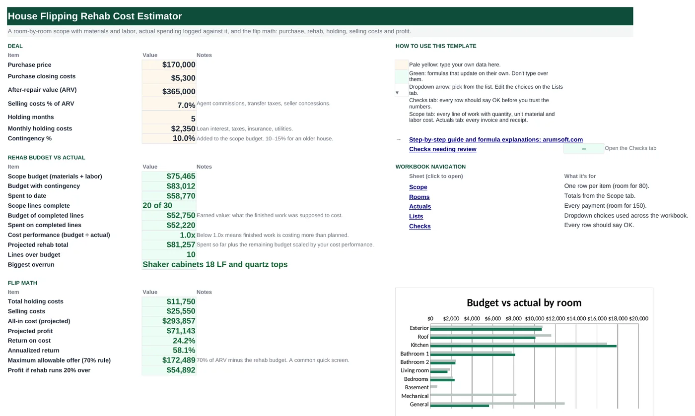
A flip is won or lost on the rehab budget. This workbook makes you write the scope line by line, with quantity, material cost and labor cost per unit, then logs every invoice against those lines so you can see which rooms and trades are over. A cost-performance index projects where the rehab will land, and the Start Here sheet turns it into profit, return on cost and the maximum allowable offer.
- Sheets:
- 6
- Works with:
- Excel for Microsoft 365, Excel 2016 or later, Excel for Mac and Excel for the web
- Updated:
What you can do with it
- Scope of work with quantity × (material + labor) per line, 30 sample lines
- Actual spending matched to scope lines by room and trade
- Budget vs actual by room and by trade, earned-value cost performance and a projected rehab total
- Flip profit, return on cost, annualized return, the 70% rule and a 20%-overrun stress test
What's inside
The workbook has 6 sheets. You only type on a few of them; the rest calculate.
| Sheet | What it's for | You enter | Calculated for you |
|---|---|---|---|
| Start Here | Deal inputs, budget vs actual summary, flip math | Price, closing costs, ARV, selling cost %, holding months and cost, contingency | Scope budget, spent, lines complete, earned value, cost performance, projected total, overruns, holding and selling costs, all-in, profit, returns, MAO, stress test |
| Scope | One row per work item (80) | Room, trade, description, quantity, unit, material and labor per unit, status | Material budget, line budget, actual, variance, used % |
| Rooms | Budget vs actual by room and by trade | Nothing | Budget, actual, variance, used % per room and per trade |
| Actuals | Every invoice and receipt (150) | Date, room, trade, vendor, type, amount, reference | Whether it matches a scope line |
| Lists | Dropdowns | Rooms, trades, units, statuses, types | Nothing |
| Checks | Six data and deal checks | Nothing | OK or Review |
Before you start
- Walk the property and list every item of work by room, with a quantity (squares of roof, feet of cabinet, square feet of floor).
- Get unit prices from your contractor or recent jobs: material per unit and labor per unit, separately.
- Decide the contingency: 10% for a cosmetic flip, 15–20% for an older house with unknowns.
Step-by-step guide
Enter the deal
Start Here B6–B12: purchase price, closing costs, ARV, selling cost %, holding months and monthly holding cost, contingency %.
Write the scope
Scope tab: room and trade from the dropdowns, a description, quantity and unit, material and labor per unit. Line budget = quantity × (material + labor).
Log every invoice
Actuals tab: date, room, trade, vendor, type, amount. The last column confirms a scope line exists for that room and trade; "No" means the money has nowhere to land.
Update statuses
Scope column M: Not started, In progress, Complete, On hold. Complete lines drive the cost-performance index.
Read the projection
Start Here B22 compares the budget of finished lines with what they actually cost; B23 scales the remaining budget by that ratio to project the final rehab total.
Read the flip math
All-in cost uses the projected rehab, holding and selling costs. Profit, return on cost and annualized return follow. B35 is the 70%-rule maximum offer; B36 shows profit if the rehab runs 20% over.
Check the Checks tab
Unmatched invoices, lines without quantity or status, a projection outside the contingency, a price above the 70% rule, and negative profit.
Formula map
Every formula in the workbook, grouped by the sheet and column it lives in. A column of copied formulas counts once; the range it covers is shown.
| Sheet | Cells | Functions | What it computes | Reads | Feeds |
|---|---|---|---|---|---|
| Scope | I5 copied down to row 84 | IF | Line budget | D5, F5, G5 | Summed on Start Here B16 and by room and trade on the Rooms tab. |
| Scope | J5 copied down to row 84 | IF, SUMIFS | Actual spent on the line | A5, B5 | Variance and used % compare it with the budget. |
| Actuals | H5 copied down to row 154 | IF, COUNTIFS | Matches a scope line? | B5, C5 | Counted on the Checks tab. |
| Start Here | B20 | SUMIF | Budget of completed lines (earned value) | — | Divided by the actual cost of the same lines for cost performance. |
| Start Here | B22 | IF | Cost performance index | B20, B21 | Scales the remaining budget in the projection. |
| Start Here | B23 | IF, OR | Projected rehab total | B22, B18, B16, B20, B17 | Feeds all-in cost and profit. |
| Start Here | B25 | IFERROR, INDEX, MATCH, MIN | Biggest overrun | — | Where to look first. |
| Start Here | B32 | arithmetic | Projected profit | B8, B31 | Return on cost divides it by all-in cost; B34 annualizes by the holding months. |
| Start Here | B35 | arithmetic | Maximum allowable offer (70% rule) | B8, B17 | Compared with the price on the Checks tab. |
| Rooms | B5 copied down to row 14 | IF, SUMIF | Budget by room | — | Charted on Start Here against actual. |
Every formula, explained
Each formula below is copied straight from the file, so what you read here is exactly what the cell contains. Click any cell in Excel to see it in the formula bar.
=IF(C5="", "", D5*(F5+G5))Quantity times the sum of material and labor per unit.
Piece by piece
D5- Quantity.
F5+G5- Material + labor per unit.
With the sample data: D5 = 28, F5 = 95, G5 = 320 → I5 result 11,620
How it is used: Summed on Start Here B16 and by room and trade on the Rooms tab.
How to change it: Nothing to change.
Learn this: How to Write Basic Formulas in Excel →=IF(C5="", "", SUMIFS(Actuals!$F$5:$F$154,
Actuals!$B$5:$B$154, A5,
Actuals!$C$5:$C$154, B5))Adds every invoice whose room and trade match this line.
Piece by piece
Actuals!$F$5:$F$154- Amounts.
Actuals!$B$5:$B$154, A5- Room matches.
Actuals!$C$5:$C$154, B5- Trade matches.
With the sample data: A5 = Roof, B5 = Roofing → J5 result 10,080.06
How it is used: Variance and used % compare it with the budget.
How to change it: If two lines share a room and trade, add a word to the trade (e.g. "Tile — floor") on both tabs so they stay separate.
Learn this: How to Use SUMIF and SUMIFS in Excel →=IF(A5="", "", IF(COUNTIFS(Scope!$A$5:$A$84, B5, Scope!$B$5:$B$84, C5)>0,
"Yes", "No"))Counts scope lines with this room and trade; at least one means the invoice will be picked up.
Piece by piece
Scope!$A$5:$A$84, B5- Room matches.
Scope!$B$5:$B$84, C5- Trade matches.
>0- At least one line.
With the sample data: B5 = Roof, C5 = Roofing → H5 result Yes
How it is used: Counted on the Checks tab.
How to change it: Nothing to change.
Learn this: How to Use COUNTIF and COUNTIFS in Excel →=SUMIF(Scope!$M$5:$M$84, "Complete", Scope!$I$5:$I$84)What the finished work was supposed to cost.
Piece by piece
Scope!$M$5:$M$84, "Complete"- Status is Complete.
Scope!$I$5:$I$84- Line budgets to add.
With the sample data: B20 result 52,750
How it is used: Divided by the actual cost of the same lines for cost performance.
How to change it: Nothing to change.
Learn this: How to Use SUMIF and SUMIFS in Excel →=IF(B21=0, "", B20/B21)Budget of completed work divided by its actual cost. 1.0 means on budget; 0.9 means every finished dollar cost $1.11.
Piece by piece
B21=0- Nothing complete yet: show nothing.
B20/B21- Earned value ÷ actual.
With the sample data: B20 = 52,750, B21 = 52,219.71 → B22 result 1.01
How it is used: Scales the remaining budget in the projection.
How to change it: Nothing to change.
Learn this: How to Use the IF Function in Excel →=IF(OR(B22="", B22=0), B17, B18+(B16-B20)/B22)Spent so far plus the remaining budget divided by the cost performance index.
Piece by piece
OR(B22="", B22=0)- No performance data yet: use the budget with contingency.
B18- Spent to date.
(B16-B20)/B22- Remaining budget, scaled by performance.
With the sample data: B22 = 1.01, B18 = 58,770.14, B16 = 75,465, B20 = 52,750, B17 = 83,011.5 → B23 result 81,256.79
How it is used: Feeds all-in cost and profit.
How to change it: Nothing to change.
Learn this: How to Use the IF Function in Excel →=IFERROR(INDEX(Scope!$C$5:$C$84,
MATCH(MIN(Scope!$K$5:$K$84), Scope!$K$5:$K$84, 0)),
"")The most negative variance on the Scope tab and the description on that row.
Piece by piece
MIN(Scope!$K$5:$K$84)- Most negative variance.
MATCH(…, Scope!$K$5:$K$84, 0)- Its row.
INDEX(Scope!$C$5:$C$84, …)- The description.
With the sample data: B25 result Shaker cabinets 18 LF and quartz tops
How it is used: Where to look first.
How to change it: Nothing to change.
Learn this: How to Use INDEX and MATCH in Excel →=B8-B31ARV minus the all-in cost.
Piece by piece
B8- After-repair value.
-B31- Purchase + closing + projected rehab + holding + selling costs.
With the sample data: B8 = 365,000, B31 = 293,856.79 → B32 result 71,143.21
How it is used: Return on cost divides it by all-in cost; B34 annualizes by the holding months.
How to change it: Nothing to change.
Learn this: How to Write Basic Formulas in Excel →=B8*0.7-B17Seventy percent of ARV minus the rehab budget with contingency: the classic quick screen for a flip.
Piece by piece
B8*0.7- 70% of ARV.
-B17- Rehab budget with contingency.
With the sample data: B8 = 365,000, B17 = 83,011.5 → B35 result 172,488.5
How it is used: Compared with the price on the Checks tab.
How to change it: Change 0.7 to 0.75 in a strong market or 0.65 for a thin one.
Learn this: How to Write Basic Formulas in Excel →=IF(A5="", "", SUMIF(Scope!$A$5:$A$84, A5, Scope!$I$5:$I$84))Adds the Scope line budgets for the room named in column A, which comes from the Lists tab.
Piece by piece
Scope!$A$5:$A$84- Room column.
A5- The room.
Scope!$I$5:$I$84- Line budgets.
With the sample data: B5 result 10,780
How it is used: Charted on Start Here against actual.
How to change it: Nothing to change; add rooms on the Lists tab.
Learn this: How to Use SUMIF and SUMIFS in Excel →Tips and limits
- Capacity: 80 scope lines, 150 invoices. Extend with Ctrl+H ($84, $154).
- Separate material and labor on every line even when one contractor quotes a lump sum; it is the only way to see which one is drifting.
- Log invoices the day they arrive and mark lines Complete when the work passes your walk-through, not when the invoice is paid. The projection depends on honest statuses.
- Holding costs are per month; every month of delay costs the sample $2,350. Put the schedule on the wall.
- The 70% rule is a screen, not a valuation. Use B32 and B36 (profit with a 20% overrun) to decide.
Learn the skills behind this template
Was this guide helpful? Spot a mistake? Send feedback · admin@arumsoft.com