HVAC and Plumbing Service Job Costing Sheet for Excel
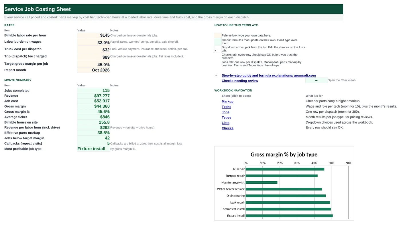
A service call that looks profitable on the invoice can lose money once drive time, labor burden and the truck are counted. This workbook prices each dispatch the way you bill it (flat rate, or hours plus a trip fee plus parts marked up by cost tier), then costs it with the technician's loaded wage for site and drive time, parts at cost and a per-call truck charge. Every job gets a gross margin and a status, and the month rolls up by technician and by job type.
- Sheets:
- 7
- Works with:
- Excel for Microsoft 365, Excel 2016 or later, Excel for Mac and Excel for the web
- Updated:
What you can do with it
- Tiered parts markup by cost, looked up automatically
- Flat-rate or time-and-materials pricing on the same log, callbacks billed at zero
- Loaded labor cost for site and drive hours, plus truck cost per dispatch
- Gross margin per job, per technician and per job type, against your target
What's inside
The workbook has 7 sheets. You only type on a few of them; the rest calculate.
| Sheet | What it's for | You enter | Calculated for you |
|---|---|---|---|
| Start Here | Rates and the month summary | Billable rate, labor burden, truck cost, trip fee, target margin, report month | Jobs, revenue, job cost, gross margin and %, average ticket, billable hours, revenue per labor hour, effective parts markup, jobs below target, callbacks, best job type |
| Markup | Parts markup tiers (10) | Cost-from thresholds and markup % | Multiplier, margin on parts |
| Techs | Technicians (15) | Name, role, hourly wage | Loaded cost per hour; jobs, hours, revenue, gross margin, GM %, callbacks for the month |
| Jobs | One row per dispatch (300) | Date, work order, customer, tech, job type, trade, pricing, hours on site, drive hours, parts cost, flat price, status | Markup tier, parts price, labor charge, trip fee, revenue, labor cost, truck cost, job cost, gross margin, GM %, margin status, month |
| Types | Results by job type (10) | Job type and trade | Jobs, revenue, gross margin, GM %, average ticket, average hours |
| Lists | Dropdowns | Pricing methods, statuses, roles | Nothing |
| Checks | Six checks | Nothing | OK or Review |
Before you start
- Know your billable hourly rate, trip fee and flat-rate prices for common jobs.
- Work out the labor burden on wages (payroll taxes, workers' comp, benefits, paid time off); 25–40% is common.
- Estimate a per-dispatch truck cost: fuel, vehicle payment and insurance, and stock shrink, divided by calls per month.
Step-by-step guide
Set the rates
Start Here B6–B11: billable rate per hour, labor burden %, truck cost per dispatch, trip fee, target gross margin, and the month to report.
Set the markup tiers
Markup tab: parts cost thresholds in ascending order with the markup for each tier. Cheap parts carry a high markup; expensive equipment a low one.
List the technicians
Techs tab: name, role, hourly wage. Loaded cost per hour = wage × (1 + burden).
Log each dispatch
Jobs tab: date, work order, customer, tech, job type, pricing method, hours on site, drive hours, parts cost, flat price (flat-rate jobs only), status. Everything to the right calculates.
Read each job
Revenue (flat rate, or labor + trip fee + marked-up parts; zero for a callback), job cost (loaded labor for site and drive, parts, truck), gross margin and a Loss / Below target / On target status.
Read the month
Start Here for the totals and the effective parts markup; the Techs tab for each technician's revenue, margin and callbacks; the Types tab for which job types and flat rates earn their keep.
Formula map
Every formula in the workbook, grouped by the sheet and column it lives in. A column of copied formulas counts once; the range it covers is shown.
| Sheet | Cells | Functions | What it computes | Reads | Feeds |
|---|---|---|---|---|---|
| Jobs | M5 copied down to row 304 | IF, LOOKUP | Markup tier | J5 | Parts price = cost × (1 + this). |
| Jobs | N5 copied down to row 304 | IF | Parts price | J5, M5 | Part of revenue on time-and-materials jobs. |
| Jobs | Q5 copied down to row 304 | IF | Revenue | L5, G5, K5, N5, O5, P5 | Gross margin = this − job cost. |
| Jobs | R5 copied down to row 304 | IF, IFERROR, INDEX, MATCH | Labor cost | H5, I5, D5 | The largest cost on most service calls. |
| Jobs | U5 copied down to row 304 | IF | Job cost | R5, S5, T5 | Subtracted from revenue for gross margin. |
| Jobs | X5 copied down to row 304 | IF | Margin status | V5, W5 | Counted on Start Here B24; colored by conditional formatting. |
| Techs | D5 copied down to row 19 | IF | Loaded cost per hour | C5 | Looked up by every job row. |
| Markup | D5 copied down to row 14 | IF | Margin on parts | B5 | A 100% markup is a 50% margin; the column keeps the two from being confused. |
| Start Here | B23 | IF, SUMIFS | Effective parts markup | — | Includes the low-markup equipment jobs, so it is lower than the top tier. |
| Types | H5 copied down to row 14 | IF, IFERROR, AVERAGEIFS | Average hours on site by job type | — | The basis for setting or checking flat-rate prices. |
Every formula, explained
Each formula below is copied straight from the file, so what you read here is exactly what the cell contains. Click any cell in Excel to see it in the formula bar.
=IF(B5="", "", LOOKUP(J5,
    Markup!$A$5:$A$14, Markup!$B$5:$B$14))
Approximate-match LOOKUP: finds the largest threshold on the Markup tab that is not more than the job's parts cost and returns that tier's markup.
Piece by piece
J5- Parts cost for the job.
Markup!$A$5:$A$14- Thresholds, ascending.
Markup!$B$5:$B$14- Markup % for each tier.
With the sample data: J5 = 125.04 → M5 result 60.0%
How it is used: Parts price = cost × (1 + this).
How to change it: Edit the tiers on the Markup tab; keep column A sorted smallest to largest.
Learn this: Lookup Formulas in Excel: XLOOKUP, VLOOKUP and INDEX/MATCH →=IF(B5="", "", J5*(1+M5))Parts cost times one plus the tier markup.
Piece by piece
J5- Parts cost.
*(1+M5)- Marked up.
With the sample data: J5 = 125.04, M5 = 60.0% → N5 result 200.06
How it is used: Part of revenue on time-and-materials jobs.
How to change it: Nothing to change.
Learn this: How to Write Basic Formulas in Excel →=IF(B5="", "", IF(L5="Callback",
0, IF(G5="Flat rate", K5, N5+O5+P5)))Zero for a callback; the flat price for a flat-rate job; otherwise marked-up parts plus labor plus the trip fee.
Piece by piece
L5="Callback"- Repeat visit: no charge.
G5="Flat rate" → K5- Flat price.
N5+O5+P5- Parts price + labor charge + trip fee.
With the sample data: L5 = Completed, G5 = Time and materials, K5 = —, N5 = 200.06, O5 = 217.5, P5 = 89 → Q5 result 506.56
How it is used: Gross margin = this − job cost.
How to change it: Nothing to change.
Learn this: How to Use the IF Function in Excel →=IF(B5="", "", (H5+I5)*IFERROR(INDEX(Techs!$D$5:$D$19, MATCH(D5, Techs!$A$5:$A$19, 0)),
0))Site plus drive hours times the technician's loaded cost per hour, looked up on the Techs tab.
Piece by piece
H5+I5- Hours on site + drive hours.
MATCH(D5, Techs!$A$5:$A$19, 0)- The tech's row.
INDEX(Techs!$D$5:$D$19, …)- Loaded cost per hour.
IFERROR(…, 0)- Zero if the name is not on the Techs tab (the Checks tab flags it).
With the sample data: H5 = 1.5, I5 = 49.0%, D5 = R. Diaz → R5 result 57.79
How it is used: The largest cost on most service calls.
How to change it: Nothing to change.
Learn this: How to Use INDEX and MATCH in Excel →=IF(B5="", "", R5+S5+T5)Labor, parts at cost and the truck.
Piece by piece
R5- Loaded labor.
+S5- Parts cost.
+T5- Truck cost per dispatch.
With the sample data: R5 = 57.79, S5 = 125.04, T5 = 32 → U5 result 214.83
How it is used: Subtracted from revenue for gross margin.
How to change it: Add a column for permits or disposal if you track them per job.
Learn this: How to Write Basic Formulas in Excel →=IF(B5="", "", IF(V5<0, "Loss",
IF(W5<'Start Here'!$B$10, "Below target", "On target")))Loss below zero; Below target under the target margin; On target otherwise.
Piece by piece
V5<0- Lost money.
W5<'Start Here'!$B$10- Under the target margin.
With the sample data: V5 = 291.73, W5 = 57.6% → X5 result On target
How it is used: Counted on Start Here B24; colored by conditional formatting.
How to change it: Change the target on Start Here.
Learn this: How to Use the IF Function in Excel →=IF(A5="", "", C5*(1+'Start Here'!$B$7))Hourly wage times one plus the labor burden.
Piece by piece
C5- Hourly wage.
*(1+'Start Here'!$B$7)- Plus taxes, insurance and benefits.
With the sample data: C5 = 38 → D5 result 50.16
How it is used: Looked up by every job row.
How to change it: Nothing to change.
Learn this: Relative, Absolute and Mixed References in Excel →=IF(A5="", "", B5/(1+B5))Markup on cost converted to margin on price: markup ÷ (1 + markup).
Piece by piece
B5- Markup %.
/(1+B5)- Divided by the multiplier.
With the sample data: B5 = 1 → D5 result 50.0%
How it is used: A 100% markup is a 50% margin; the column keeps the two from being confused.
How to change it: Nothing to change.
Learn this: How to Write Basic Formulas in Excel →=IF(SUMIFS(Jobs!$J$5:$J$304,
Jobs!$Y$5:$Y$304, B11)=0,
0, SUMIFS(Jobs!$N$5:$N$304,
Jobs!$Y$5:$Y$304, B11)/SUMIFS(Jobs!$J$5:$J$304,
Jobs!$Y$5:$Y$304, B11)-1)Parts price billed in the month divided by parts cost, minus one: the markup you actually achieved across all tiers.
Piece by piece
SUMIFS(Jobs!$N…, Jobs!$Y…, B11)- Parts price for the month.
SUMIFS(Jobs!$J…, Jobs!$Y…, B11)- Parts cost for the month.
…/…-1- Achieved markup.
With the sample data: B23 result 38.5%
How it is used: Includes the low-markup equipment jobs, so it is lower than the top tier.
How to change it: Nothing to change.
Learn this: How to Use SUMIF and SUMIFS in Excel →=IF(A5="", "", IFERROR(AVERAGEIFS(Jobs!$H$5:$H$304, Jobs!$E$5:$E$304, A5, Jobs!$Y$5:$Y$304, 'Start Here'!$B$11),
""))Average of hours on site for jobs of this type in the report month.
Piece by piece
Jobs!$H$5:$H$304- Hours on site.
Jobs!$E$5:$E$304, A5- Job type matches.
Jobs!$Y$5:$Y$304, 'Start Here'!$B$11- Report month.
IFERROR(…, "")- Blank if no jobs.
With the sample data: H5 result 2.3
How it is used: The basis for setting or checking flat-rate prices.
How to change it: Nothing to change.
Learn this: How to Use AVERAGEIF and AVERAGEIFS in Excel →Tips and limits
- Capacity: 300 jobs, 15 technicians, 10 markup tiers, 10 job types. Start a new file each quarter, or extend with Ctrl+H ($304).
- Watch the maintenance visit line: in the sample a $169 flat rate barely covers a senior tech, an hour of drive time and the truck. Flat rates must be priced on loaded cost, not wage.
- Drive time is a real cost even when the customer never sees it. Route planning raises revenue per labor hour as much as a price increase.
- A callback is billed at zero, so every callback is pure margin loss; the Techs tab counts them per person.
- Warranty work can use the "Warranty (no charge)" pricing method; add a revenue formula for any manufacturer labor allowance you receive.
Learn the skills behind this template
Was this guide helpful? Spot a mistake? Send feedback · admin@arumsoft.com