Recruiting Pipeline Tracker for Excel (Time to Fill and Cost per Hire)
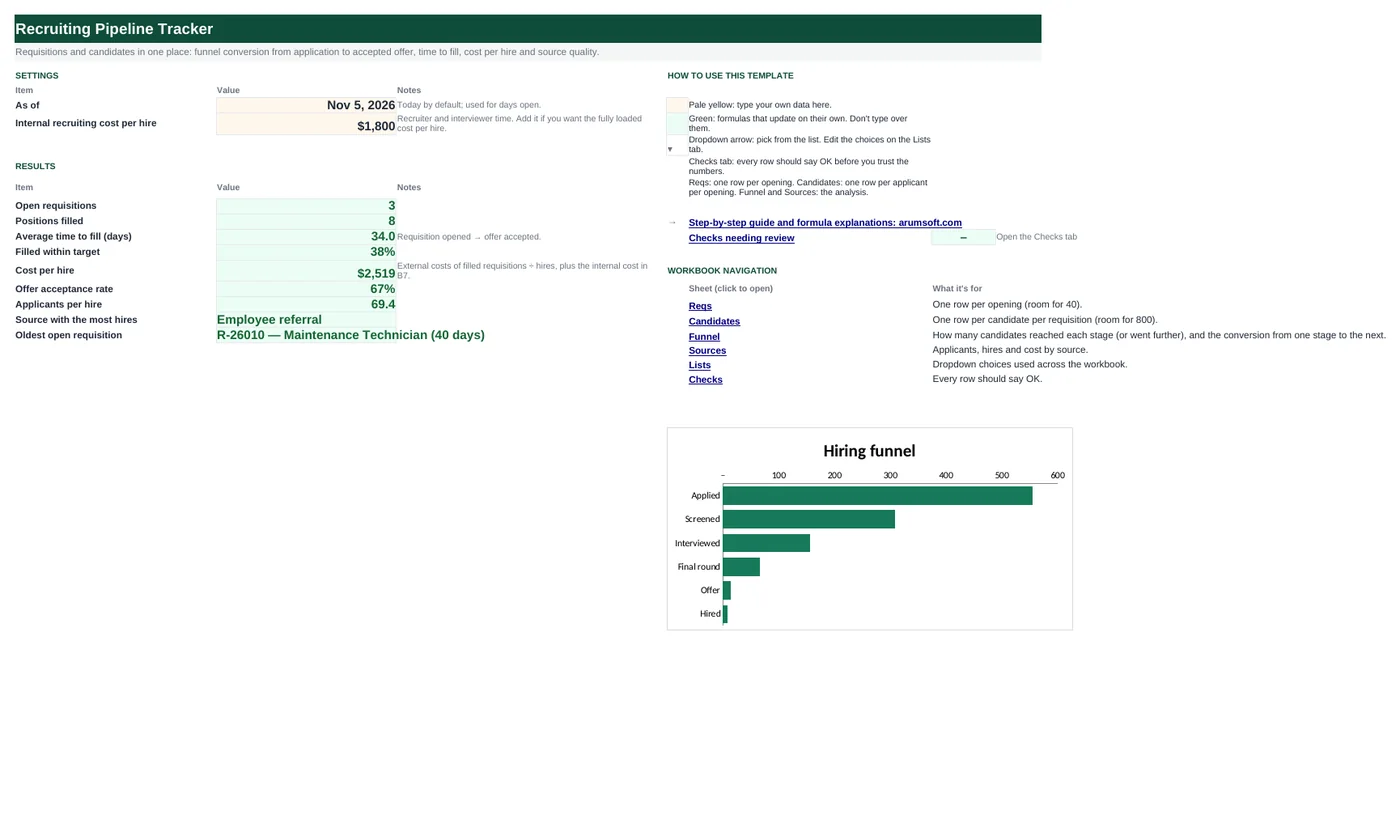
Recruiting gets better when you can see where candidates drop out, which sources produce hires and how long each opening really takes. This workbook keeps two simple lists: requisitions and candidates. For each candidate you record the source, the furthest stage reached and the outcome. From that it builds the funnel with conversion at every step, time to fill for every requisition against its target, cost per hire, offer acceptance and the cost and hire rate of every source.
- Sheets:
- 7
- Works with:
- Excel for Microsoft 365, Excel 2016 or later, Excel for Mac and Excel for the web
- Updated:
What you can do with it
- Requisitions with fill date from the hired candidate, time to fill, days open and status against target
- External cost per requisition (ads, agency, referral bonus) plus your internal cost per hire
- Hiring funnel: candidates reaching each stage and conversion from the previous stage and from applied
- Source quality: applicants, hires, applicant-to-hire rate, interview rate and cost per hire
What's inside
The workbook has 7 sheets. You only type on a few of them; the rest calculate.
| Sheet | What it's for | You enter | Calculated for you |
|---|---|---|---|
| Start Here | Settings and KPIs | As-of date (today), internal cost per hire | Open and filled, time to fill, on-target %, cost per hire, offer acceptance, applicants per hire, top source, oldest open |
| Reqs | One row per opening (40) | Req ID, title, department, hiring manager, recruiter, opened, target days, status, ads, agency fee, referral bonus, other | Filled on, time to fill, days open, vs target, applicants, external cost |
| Candidates | One row per candidate per req (800) | Candidate, req, source, applied, furthest stage, outcome, hire date | Stage number, consistency check |
| Funnel | Stage counts and conversion | Nothing | Reached, from previous stage, from applied |
| Sources | By source | Source and its spend for the period | Applicants, hires, hire rate, interview rate, cost per hire |
| Lists | Dropdowns | Stages, outcomes, statuses, departments | Nothing |
| Checks | Six data checks | Nothing | OK or Review |
Before you start
- Agree the stage names and what moves a candidate into each one.
- Set a target time to fill for each type of role (hourly roles are often 2–4 weeks, senior roles 6–10).
- Collect spend per source for the same period: job board subscriptions, campus events, agency fees.
Step-by-step guide
Set the internal cost
Start Here B7: recruiter and interviewer time per hire, if you want fully loaded cost per hire.
Open requisitions
Reqs tab: ID, title, department, hiring manager, recruiter, opened date, target days, status and external costs.
Log candidates
Candidates tab: one row per candidate per req with source, applied date, furthest stage and outcome. For the hire, enter the hire date.
Read the funnel
Funnel tab: where candidates drop out. A steep drop from Interviewed to Final round points at screening quality.
Compare sources
Sources tab: which sources produce hires, not just applicants, and at what cost.
Watch the open reqs
Reqs column L flags requisitions past their target; Start Here shows the oldest.
Formula map
Every formula in the workbook, grouped by the sheet and column it lives in. A column of copied formulas counts once; the range it covers is shown.
| Sheet | Cells | Functions | What it computes | Reads | Feeds |
|---|---|---|---|---|---|
| Reqs | I5 copied down to row 44 | IF, COUNTIFS, MINIFS | Filled on | A5 | Time to fill = filled on − opened. |
| Reqs | L5 copied down to row 44 | IF | vs target | J5, G5, K5 | Start Here B14 is the share filled on target. |
| Reqs | Q5 copied down to row 44 | IF | External cost | N5, O5, P5, R5 | Cost per hire on Start Here = total of filled reqs ÷ hires. |
| Candidates | H5 copied down to row 804 | IF, MATCH | Stage number | E5 | The funnel counts candidates at or beyond each number. |
| Funnel | B7 | COUNTIF | Reached a stage | — | Conversion = this ÷ previous stage; also ÷ applied. |
| Funnel | C7 copied down to row 10 | IF | Conversion from the previous stage | B7, B6 | The weakest step is where to look first. |
| Start Here | B16 | IFERROR, COUNTIF | Offer acceptance rate | — | Low acceptance usually points at pay, speed or the candidate experience. |
| Sources | G5 copied down to row 14 | IF, SUMPRODUCT, SUMIF | Cost per hire by source | — | Compare with applicant-to-hire rate before cutting a source. |
Every formula, explained
Each formula below is copied straight from the file, so what you read here is exactly what the cell contains. Click any cell in Excel to see it in the formula bar.
=IF(A5="", "", IF(COUNTIFS(Candidates!$B$5:$B$804, A5, Candidates!$F$5:$F$804, "Hired")=0,
    "", MINIFS(Candidates!$G$5:$G$804, Candidates!$B$5:$B$804, A5, Candidates!$F$5:$F$804, "Hired")))
The hire date of the candidate marked Hired for this requisition.
Piece by piece
MINIFS(Candidates!$G$5:$G$804, Candidates!$B$5:$B$804, A5, Candidates!$F$5:$F$804, "Hired")- Hire date for this req.
COUNTIFS(…)=0- No hire yet: blank.
With the sample data: A5 = R-26001 → I5 result Jul 4, 2026
How it is used: Time to fill = filled on − opened.
How to change it: Nothing to change.
Learn this: How to Use MIN and MAX in Excel →=IF(A5="", "", IF(J5<>"",
IF(J5<=G5, "On target", "Late"),
IF(H5="Open", IF(K5>G5, "Past target", "Open"), "")))For filled reqs, On target or Late; for open reqs, Past target once days open exceed the target.
Piece by piece
J5<>""- Filled: compare time to fill with target.
H5="Open"- Open: compare days open with target.
With the sample data: J5 = 34, G5 = 45, K5 = — → L5 result On target
How it is used: Start Here B14 is the share filled on target.
How to change it: Change target days per req in column G.
Learn this: How to Use the IF Function in Excel →=IF(A5="", "", N5+O5+P5+R5+IF(H5="Filled",
'Start Here'!$B$7, 0))Ads, agency fee, referral bonus and other costs, plus the internal cost per hire if the req is filled.
Piece by piece
N5+O5+P5+R5- External costs.
IF(H5="Filled", 'Start Here'!$B$7, 0)- Internal cost per hire.
With the sample data: N5 = 400, O5 = 0, P5 = 500, R5 = 0 → Q5 result 2,700
How it is used: Cost per hire on Start Here = total of filled reqs ÷ hires.
How to change it: Set B7 to 0 for external cost only.
Learn this: How to Write Basic Formulas in Excel →=IF(E5="", "", MATCH(E5, Lists!$A$5:$A$10, 0))Position of the furthest stage in the stage list: Applied 1 … Hired 6.
Piece by piece
MATCH(E5, Lists!$A$5:$A$10, 0)- Exact position.
With the sample data: E5 = Applied → H5 result 1
How it is used: The funnel counts candidates at or beyond each number.
How to change it: Edit stage names on the Lists tab (keep them in order).
Learn this: How to Use INDEX and MATCH in Excel →=COUNTIF(Candidates!$H$5:$H$804, ">="&3)Candidates whose furthest stage is this one or later.
Piece by piece
COUNTIF(Candidates!$H$5:$H$804, ">="&3)- Stage 3 (Interviewed) or beyond.
With the sample data: B7 result 156
How it is used: Conversion = this ÷ previous stage; also ÷ applied.
How to change it: Nothing to change.
Learn this: How to Use COUNTIF and COUNTIFS in Excel →=IF(B6=0, "", B7/B6)Share of candidates who reached the previous stage and went on to this one.
Piece by piece
B7/B6- Interviewed ÷ screened.
With the sample data: B7 = 156, B6 = 308 → C7 result 50.6%
How it is used: The weakest step is where to look first.
How to change it: Nothing to change.
Learn this: How to Write Basic Formulas in Excel →=IFERROR(COUNTIF(Candidates!$F$5:$F$804,
"Hired")/(COUNTIF(Candidates!$F$5:$F$804, "Hired")+COUNTIF(Candidates!$F$5:$F$804, "Declined offer")),
0)Hires ÷ (hires + offers declined).
Piece by piece
COUNTIF(Candidates!$F$5:$F$804, "Hired")- Accepted offers.
+COUNTIF(…, "Declined offer")- Plus declined.
With the sample data: B16 result 66.7%
How it is used: Low acceptance usually points at pay, speed or the candidate experience.
How to change it: Nothing to change.
Learn this: How to Use COUNTIF and COUNTIFS in Excel →=IF(N(D5)=0, "", (B5+SUMPRODUCT((Candidates!$C$5:$C$804=A5)*(Candidates!$F$5:$F$804="Hired")*SUMIF(Reqs!$A$5:$A$44, Candidates!$B$5:$B$804, Reqs!$O$5:$O$44)))/D5)The source's spend plus agency fees on the requisitions its hires filled, divided by its hires.
Piece by piece
B5- Spend for the period.
(Candidates!$C$5:$C$804=A5)*(Candidates!$F$5:$F$804="Hired")- 1 for this source's hires.
SUMIF(Reqs!$A$5:$A$44, Candidates!$B$5:$B$804, Reqs!$O$5:$O$44)- Agency fee on each candidate's req (SUMIF as a lookup).
SUMPRODUCT(…)/D5- Added and divided by hires.
With the sample data: G5 result 3,000
How it is used: Compare with applicant-to-hire rate before cutting a source.
How to change it: Nothing to change.
Learn this: How to Use SUMIF and SUMIFS in Excel →Tips and limits
- Capacity: 40 requisitions and 800 candidate rows.
- Time to fill here runs from requisition opened to offer accepted (hire date). If you measure to start date, enter the start date as the hire date.
- Record the furthest stage, not the current one; a rejected finalist stays at Final round.
- Referral and careers-page hires look free in source spend; add referral bonuses and your careers-site cost to see the real comparison.
- B6 is =TODAY(), so days open grow every day.
Learn the skills behind this template
Was this guide helpful? Spot a mistake? Send feedback · admin@arumsoft.com