BRRRR Real Estate Calculator for Excel
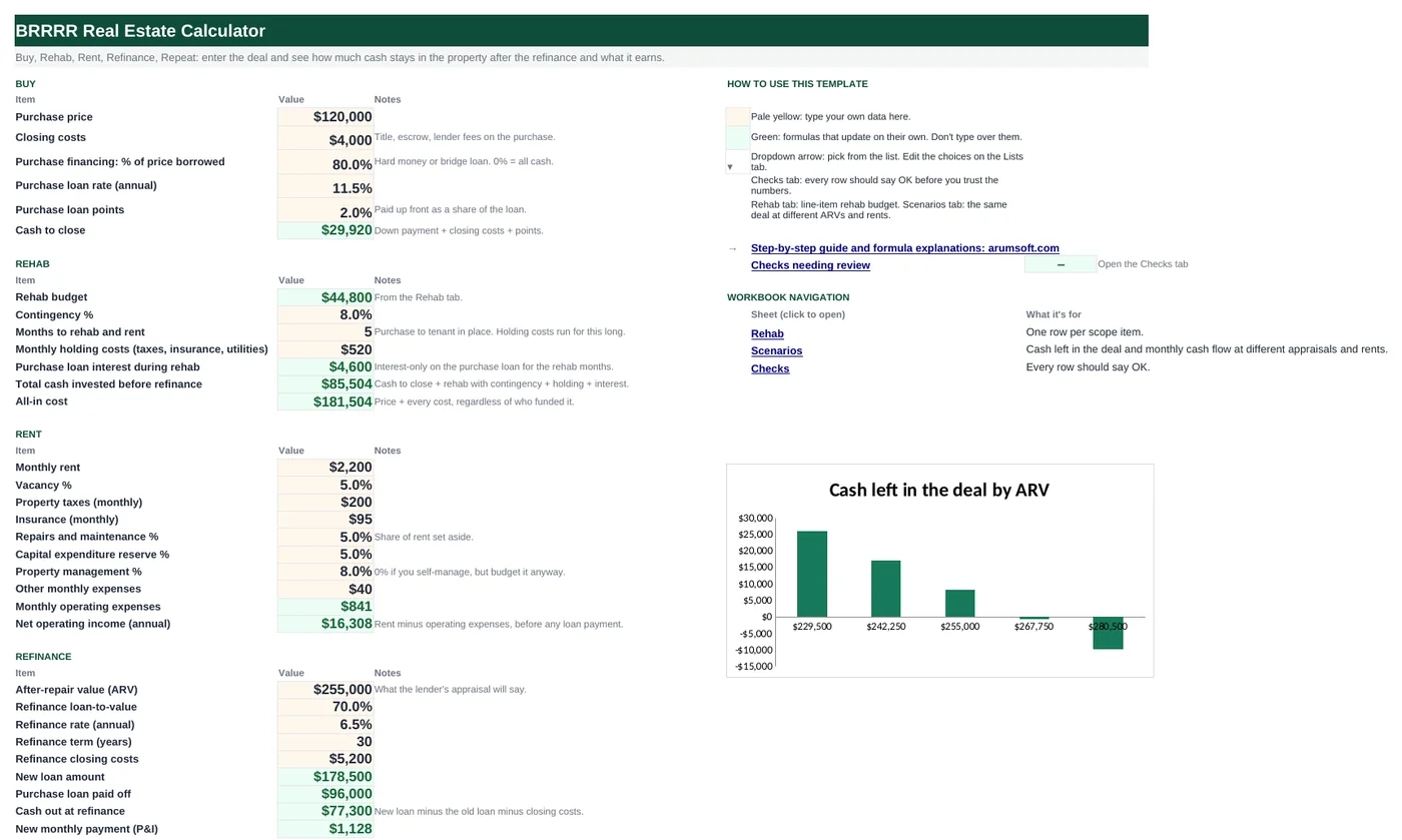
The BRRRR strategy only works if the refinance returns most of the cash you put in. This workbook follows the deal through all four steps, with a line-item rehab budget, interest and holding costs for the months the property is empty, operating expenses as percentages of rent, and a refinance at the after-repair value. It ends with cash left in the deal, monthly cash flow on the new loan, cash-on-cash return and DSCR, plus a scenario grid for lower appraisals and rents.
- Sheets:
- 4
- Works with:
- Excel for Microsoft 365, Excel 2016 or later, Excel for Mac and Excel for the web
- Updated:
What you can do with it
- Total cash invested before the refinance, including points, interest and holding costs
- Cash out at refinance and the cash left in the deal
- Cash flow, cash-on-cash and DSCR on the new loan
- A max purchase price for a full cash-out, and ARV/rent scenarios
What's inside
The workbook has 4 sheets. You only type on a few of them; the rest calculate.
| Sheet | What it's for | You enter | Calculated for you |
|---|---|---|---|
| Start Here | The whole deal on one sheet | Price, closing costs, loan terms, contingency, months, holding costs, rent and expense assumptions, ARV and refinance terms | Cash to close, cash invested, NOI, new loan and payment, cash out, cash left in, cash flow, cash-on-cash, DSCR, equity, max price, deal check |
| Rehab | Line-item rehab budget (12 rows) | Scope item and estimate | Total, total with contingency, rehab as % of price |
| Scenarios | ARV and rent from −10% to +10% | Nothing (edit the multipliers if you like) | Loan, cash out, cash left in, cash flow, cash-on-cash, DSCR per row |
| Checks | Six deal checks | Nothing | OK or Review |
Before you start
- Get a realistic after-repair value from comparable sales, not from the listing agent.
- Walk the property with a contractor and write the rehab scope line by line.
- Know your refinance lender's terms: LTV (70–75% is common), rate, seasoning period, and the DSCR they require.
Step-by-step guide
Enter the purchase
Price, closing costs, how much of the price is borrowed (hard money or a bridge loan), its rate and points. Cash to close calculates.
Build the rehab budget
Rehab tab: one row per scope item. The total flows to Start Here B15; the contingency in B16 is added on top.
Set the timeline and holding costs
Months from purchase to a tenant in place (B17) and monthly holding costs (B18). Interest on the purchase loan is calculated for those months.
Enter rent and expenses
Monthly rent, vacancy, taxes, insurance, repairs, capex and management as a share of rent. NOI is annual rent minus operating expenses.
Enter the refinance
ARV, the lender's LTV, rate, term and closing costs. The new loan, the payoff of the purchase loan and the cash out calculate.
Read the results
Cash left in the deal is what you still have invested. Cash flow is after the new payment. The deal check needs little cash left in, positive cash flow and DSCR ≥ 1.2.
Stress it on the Scenarios tab
The same deal with the appraisal and rent 5% and 10% lower or higher. The Checks tab adds the 1% rule, DSCR and LTV sanity checks.
Formula map
Every formula in the workbook, grouped by the sheet and column it lives in. A column of copied formulas counts once; the range it covers is shown.
| Sheet | Cells | Functions | What it computes | Reads | Feeds |
|---|---|---|---|---|---|
| Start Here | B11 | arithmetic | Cash to close | B6, B8, B7, B10 | The first piece of total cash invested. |
| Start Here | B19 | arithmetic | Purchase loan interest during rehab | B6, B8, B9, B17 | Added to cash invested; hard-money interest is a real cost many first-timers forget. |
| Start Here | B20 | arithmetic | Total cash invested before refinance | B11, B15, B16, B18, B17, B19 | Cash left in the deal is this minus the cash out. |
| Start Here | B33 | arithmetic | Monthly operating expenses | B25, B26, B29, B30, B31, B27, B28, B32 | NOI and cash flow subtract this from rent. |
| Start Here | B45 | arithmetic | Cash out at refinance | B43, B44, B42 | Subtracted from cash invested to give cash left in the deal. |
| Start Here | B46 | IF, PMT | New monthly payment | B40, B41, B43 | Cash flow after refinance subtracts this from rent and expenses. |
| Start Here | B52 | IF | Cash-on-cash return | B51, B50 | The headline return on the deal. |
| Start Here | B57 | arithmetic | Max purchase price for a full cash-out | B45, B6, B20 | A quick negotiating anchor. |
| Start Here | B58 | IF, AND, OR | Deal check | B50, B20, B51, B53 | A plain-language verdict on the dashboard. |
| Scenarios | F5 copied down to row 9 | IF, PMT | Cash flow in a scenario | E5, B5 | Columns G and H turn it into cash-on-cash and DSCR. |
Every formula, explained
Each formula below is copied straight from the file, so what you read here is exactly what the cell contains. Click any cell in Excel to see it in the formula bar.
=B6*(1-B8)+B7+B6*B8*B10The down payment, closing costs and the points on the purchase loan.
Piece by piece
B6*(1-B8)- Price × the share not borrowed = down payment.
+B7- Closing costs.
+B6*B8*B10- Loan amount × points.
With the sample data: B6 = 120,000, B8 = 80.0%, B7 = 4,000, B10 = 2.0% → B11 result 29,920
How it is used: The first piece of total cash invested.
How to change it: Nothing to change.
Learn this: How to Write Basic Formulas in Excel →=B6*B8*B9/12*B17Interest-only on the purchase loan for the months until the property is rented.
Piece by piece
B6*B8- Loan amount.
*B9/12- Monthly interest rate.
*B17- Months to rehab and rent.
With the sample data: B6 = 120,000, B8 = 80.0%, B9 = 11.5%, B17 = 5 → B19 result 4,600
How it is used: Added to cash invested; hard-money interest is a real cost many first-timers forget.
How to change it: If your lender charges interest on the rehab draw too, add it here.
Learn this: How to Write Basic Formulas in Excel →=B11+B15*(1+B16)+B18*B17+B19Everything you paid out of pocket up to the refinance.
Piece by piece
B11- Cash to close.
+B15*(1+B16)- Rehab budget with contingency.
+B18*B17- Holding costs × months.
+B19- Purchase loan interest.
With the sample data: B11 = 29,920, B15 = 44,800, B16 = 8.0%, B18 = 520, B17 = 5, B19 = 4,600 → B20 result 85,504
How it is used: Cash left in the deal is this minus the cash out.
How to change it: Nothing to change.
Learn this: How to Write Basic Formulas in Excel →=B25*(B26+B29+B30+B31)+B27+B28+B32The percentage-of-rent items are summed and applied to rent, then the fixed items are added.
Piece by piece
B25*(B26+B29+B30+B31)- Rent × (vacancy + repairs + capex + management).
+B27+B28+B32- Taxes, insurance, other.
With the sample data: B25 = 2,200, B26 = 5.0%, B29 = 5.0%, B30 = 5.0%, B31 = 8.0%, B27 = 200, B28 = 95, B32 = 40 → B33 result 841
How it is used: NOI and cash flow subtract this from rent.
How to change it: Nothing to change; add an item to B32.
Learn this: How to Write Basic Formulas in Excel →=B43-B44-B42The new loan pays off the purchase loan and the refinance closing costs; what is left comes back to you.
Piece by piece
B43- New loan = ARV × LTV.
-B44- Purchase loan paid off.
-B42- Refinance closing costs.
With the sample data: B43 = 178,500, B44 = 96,000, B42 = 5,200 → B45 result 77,300
How it is used: Subtracted from cash invested to give cash left in the deal.
How to change it: Nothing to change.
Learn this: How to Write Basic Formulas in Excel →=IF(B43=0, 0, -PMT(B40/12, B41*12, B43))Principal and interest on the refinance loan. PMT returns a negative number for a payment, so the minus sign in front makes it positive.
Piece by piece
B40/12- Monthly rate.
B41*12- Number of payments.
B43- Loan amount.
-PMT(…)- Flip the sign.
With the sample data: B40 = 6.5%, B41 = 30, B43 = 178,500 → B46 result 1,128.24
How it is used: Cash flow after refinance subtracts this from rent and expenses.
How to change it: For an interest-only loan use B43*B40/12.
Learn this: Essential Excel Functions: SUM, AVERAGE, COUNT, MIN and MAX →=IF(B50<=0, "Infinite", B51*12/B50)Annual cash flow divided by the cash still invested. When nothing is left in, the return is infinite, which is the point of BRRRR.
Piece by piece
B50<=0- Nothing (or less) left in the deal.
"Infinite"- Shown instead of dividing by zero or a negative.
B51*12/B50- Annual cash flow ÷ cash left in.
With the sample data: B51 = 230.76, B50 = 8,204 → B52 result 33.8%
How it is used: The headline return on the deal.
How to change it: Nothing to change.
Learn this: How to Use the IF Function in Excel →=B45+B6-B20The price at which cash out would exactly equal cash invested. Every other input stays as entered, so a lower price also lowers the cash to close and the loan (handled algebraically here as a simple shift).
Piece by piece
B45- Cash out at the current price.
+B6- Current price.
-B20- Current cash invested.
With the sample data: B45 = 77,300, B6 = 120,000, B20 = 85,504 → B57 result 111,796
How it is used: A quick negotiating anchor.
How to change it: Nothing to change.
Learn this: How to Write Basic Formulas in Excel →=IF(AND(B50<=B20*0.1, B51>=100,
OR(B53="", B53>=1.2)), "Strong",
IF(AND(B51>=0, OR(B53="", B53>=1)),
"Workable", "Weak"))Three tests: little cash left in (≤10% of what you invested), at least $100 a month cash flow, and DSCR of 1.2 or more.
Piece by piece
B50<=B20*0.1- Cash left in is 10% or less of cash invested.
B51>=100- Monthly cash flow at least $100.
OR(B53="", B53>=1.2)- DSCR 1.2+ (or no loan).
AND(…) → "Strong"- All three pass.
AND(B51>=0, DSCR>=1.0) → "Workable"- Fallback test.
With the sample data: B50 = 8,204, B20 = 85,504, B51 = 230.76, B53 = 1.2 → B58 result Strong
How it is used: A plain-language verdict on the dashboard.
How to change it: Change the thresholds to your own criteria.
Learn this: How to Use AND and OR in Excel →=E5-(E5*('Start Here'!$B$26+'Start Here'!$B$29+'Start Here'!$B$30+'Start Here'!$B$31)+'Start Here'!$B$27+'Start Here'!$B$28+'Start Here'!$B$32)-IF(B5=0,
0, -PMT('Start Here'!$B$40/12,
'Start Here'!$B$41*12, B5))The full cash flow formula for one row: the row's rent, minus operating expenses built from the Start Here percentages, minus the payment on the row's loan.
Piece by piece
E5*('Start Here'!$B$26+…+$B$31)- Percentage expenses on this row's rent.
+'Start Here'!$B$27+$B$28+$B$32- Fixed expenses.
-PMT('Start Here'!$B$40/12, $B$41*12, B5)- Payment on this row's loan amount.
With the sample data: E5 = 1,980, B5 = 160,650 → F5 result 174.18
How it is used: Columns G and H turn it into cash-on-cash and DSCR.
How to change it: Nothing to change.
Learn this: Relative, Absolute and Mixed References in Excel →Tips and limits
- Appraisals come in low more often than high. Run the deal at 90% of your ARV before you offer; if it still works, you have a margin of safety.
- Most refinance lenders require a seasoning period (6–12 months of ownership) before they lend on the appraised value. Add those months to B17 if you cannot refinance sooner.
- Hard-money points and interest are the hidden cost of BRRRR; the sample loses $6,500 to them. A private lender at a lower rate changes the deal a lot.
- Cash-on-cash on a tiny amount left in looks huge (the sample shows 34%). The better test is whether the property cash flows on its own with the new loan (B51) and whether DSCR satisfies the lender.
- Use the Rehab tab honestly. The budget with contingency is the number that decides whether the refinance covers you.
Learn the skills behind this template
Was this guide helpful? Spot a mistake? Send feedback · admin@arumsoft.com