DSCR Loan Calculator for Excel
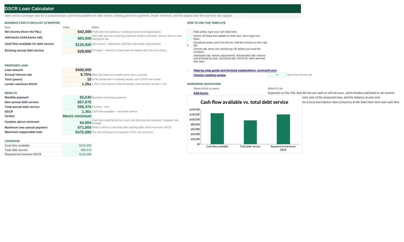
Before you apply for a term loan, see the number the lender will compute first. Enter net income, the add-backs lenders accept, your existing payments and the proposed loan terms; the workbook gives the DSCR, a pass/fail against the lender's minimum, the cushion, and the largest loan your cash flow supports. An amortization tab shows interest and principal by year and a sensitivity grid shows DSCR for other amounts and rates.
- Sheets:
- 5
- Works with:
- Excel for Microsoft 365, Excel 2016 or later, Excel for Mac and Excel for the web
- Updated:
What you can do with it
- Compute cash flow available for debt service from net income and add-backs
- See the DSCR for a proposed loan against a 1.25x (or your lender's) minimum
- Find the maximum loan your cash flow supports at a given rate and term
- Check interest and principal by year, and DSCR across amounts and rates
What's inside
The workbook has 5 sheets. You only type on a few of them; the rest calculate.
| Sheet | What it's for | You enter | Calculated for you |
|---|---|---|---|
| Start Here | Inputs, results and a coverage chart | Net income, existing debt service, loan amount, rate, term, lender minimum | Add-backs total, cash flow available, payment, new and total debt service, DSCR, verdict, cushion, maximum payment and loan |
| Add-backs | Itemized lender adjustments (20 rows) | Add-back, amount, reason | Total |
| Amortization | Year-by-year interest, principal and balance (25 years) | Nothing | Payments, interest (CUMIPMT), principal (CUMPRINC), ending balance, DSCR that year |
| Sensitivity | DSCR grid: loan amount × interest rate | The amounts and rates on the edges | Every DSCR in the grid, colored against the minimum |
| Checks | Six checks | Nothing | OK or Review |
Before you start
- Use the last full fiscal year (or trailing twelve months) from your P&L. Lenders will ask for the same period.
- List add-backs honestly: depreciation, amortization, interest on existing loans, and non-recurring or owner-related expenses you can document.
- Existing debt service is the annual principal plus interest on loans that will still be there after the new one closes; leave out any loan the new one refinances.
Step-by-step guide
Enter cash flow
Start Here B6 is net income from the P&L. B7 pulls the Add-backs tab total; itemize there. B8, cash flow available for debt service, is the lender's numerator.
Enter existing debt service
B9: the annual payments that remain after this loan. Refinanced loans drop out.
Enter the proposed loan
B12 amount, B13 annual rate, B14 term in years, B15 the lender's minimum DSCR (1.25x for most SBA 7(a) lenders).
Read the results
The monthly payment comes from PMT; annual debt service is 12 payments; total adds existing. DSCR is B8 ÷ B20. The verdict compares with the minimum, the cushion says how much cash flow could fall, and the maximum supportable loan uses PV to turn the spare payment capacity into a loan amount.
Check the Amortization tab
Interest and principal for each year of the loan, the ending balance and the DSCR each year if cash flow stays flat. Lenders look at year one; you should look at the whole term.
Use the Sensitivity tab
DSCR for eight loan amounts against eight rates at your term. Green cells meet the minimum. Edit the yellow edge values for your own ranges.
Check the Checks tab
Terms entered, rate as a percentage, term within 25 years, amortization principal tying to the loan, add-backs described, and DSCR meeting the minimum.
Formula map
Every formula in the workbook, grouped by the sheet and column it lives in. A column of copied formulas counts once; the range it covers is shown.
| Sheet | Cells | Functions | What it computes | Reads | Feeds |
|---|---|---|---|---|---|
| Start Here | B18 | IF, OR, PMT | Monthly payment | B12, B13, B14 | Annual debt service in B19 is 12 of these. |
| Start Here | B21 | IF | DSCR | B8, B20 | The verdict and the Checks tab compare it with B15. |
| Start Here | B22 | IF | Verdict | B21, B15 | A one-line answer for the loan discussion. |
| Start Here | B23 | arithmetic | Cushion above minimum | B8, B20, B15 | Negative means the shortfall you would need to close. |
| Start Here | B24 | MAX | Maximum new annual payment | B8, B15, B9 | B25 converts it to a loan amount. |
| Start Here | B25 | IF, PV | Maximum supportable loan | B24 | The upper bound to discuss with the lender. |
| Amortization | C5 copied down to row 29 | IF, CUMIPMT | Interest paid in a year | A5 | Ending balance in E5 subtracts cumulative principal from the loan. |
| Amortization | F5 copied down to row 29 | IF | DSCR in a given year | — | Shows coverage over the life of the loan. |
| Sensitivity | B5 copied down to row 12 | IF, PMT | DSCR for one amount and rate | — | Colored green at or above the minimum, red below 1.0x. |
| Checks | B8 | IF, ABS | Amortization ties to the loan | — | A mismatch means the term exceeds the 25-year table. |
Every formula, explained
Each formula below is copied straight from the file, so what you read here is exactly what the cell contains. Click any cell in Excel to see it in the formula bar.
=IF(OR(B12=0, B14=0), 0, -PMT(B13/12, B14*12, B12))Excel's PMT returns the level payment that repays the loan over the term. It is negative by convention (money going out), so the formula negates it.
Piece by piece
B13/12- Monthly rate: annual rate ÷ 12.
B14*12- Number of monthly payments.
B12- Loan amount (present value).
-PMT(…)- Flip the sign so the payment shows positive.
With the sample data: B12 = 450,000, B13 = 8.8%, B14 = 10 → B18 result 5,639.7
How it is used: Annual debt service in B19 is 12 of these.
How to change it: For interest-only periods, model them on the Amortization tab instead.
Learn this: How to Write Basic Formulas in Excel →=IF(B20=0, 0, B8/B20)Cash flow available divided by total annual debt service. 1.0x means cash flow exactly covers payments; lenders want a margin above that.
Piece by piece
B20=0- No debt service: show 0 rather than an error.
B8/B20- Cash flow available ÷ (existing + new debt service).
With the sample data: B8 = 125,500, B20 = 96,476.45 → B21 result 1.3
How it is used: The verdict and the Checks tab compare it with B15.
How to change it: Nothing to change.
Learn this: How to Write Basic Formulas in Excel →=IF(B21>=B15, "Meets minimum",
IF(B21>=1, "Below lender minimum",
"Cannot cover payments"))Three outcomes: meets the lender minimum, covers payments but below the minimum, or cannot cover payments (below 1.0x).
Piece by piece
B21>=B15- At or above the minimum.
B21>=1- Between 1.0x and the minimum.
"Cannot cover payments"- Below 1.0x.
With the sample data: B21 = 1.3, B15 = 1.25 → B22 result Meets minimum
How it is used: A one-line answer for the loan discussion.
How to change it: Nothing to change.
Learn this: How to Use the IF Function in Excel →=B8-B20*B15How much cash flow available could fall before DSCR drops to the minimum: cash flow minus (debt service × minimum).
Piece by piece
B20*B15- The cash flow needed to hit exactly the minimum DSCR.
B8-…- What you have above that.
With the sample data: B8 = 125,500, B20 = 96,476.45, B15 = 1.25 → B23 result 4,904.44
How it is used: Negative means the shortfall you would need to close.
How to change it: Nothing to change.
Learn this: How to Write Basic Formulas in Excel →=MAX(0, B8/B15-B9)At the minimum DSCR, total debt service can be at most cash flow ÷ minimum. Subtract existing payments to get what is left for a new loan.
Piece by piece
B8/B15- Largest total debt service allowed.
-B9- Less existing debt service.
MAX(0, …)- Never negative.
With the sample data: B8 = 125,500, B15 = 1.25, B9 = 28,800 → B24 result 71,600
How it is used: B25 converts it to a loan amount.
How to change it: Nothing to change.
Learn this: How to Use MIN and MAX in Excel →=IF(B24=0, 0, PV(B13/12, B14*12, -B24/12))PV turns a monthly payment into the loan it would repay at the given rate and term. The payment is divided by 12 and negated because PV expects an outflow.
Piece by piece
B13/12, B14*12- Monthly rate and number of payments.
-B24/12- The monthly payment capacity, as an outflow.
PV(…)- The loan amount that payment supports.
With the sample data: B24 = 71,600 → B25 result 476,088.84
How it is used: The upper bound to discuss with the lender.
How to change it: Nothing to change.
Learn this: How to Write Basic Formulas in Excel →=IF(A5>'Start Here'!$B$14,
"", -CUMIPMT('Start Here'!$B$13/12,
'Start Here'!$B$14*12, 'Start Here'!$B$12,
(A5-1)*12+1, A5*12, 0))CUMIPMT returns the interest paid between two payment numbers. Year y covers payments (y−1)×12+1 through y×12. Negative by convention, so it is negated. Column D does the same with CUMPRINC for principal.
Piece by piece
'Start Here'!$B$13/12, 'Start Here'!$B$14*12, 'Start Here'!$B$12- Monthly rate, number of payments, loan amount.
(A5-1)*12+1, A5*12- First and last payment of the year.
0- Payments at the end of each period.
IF(A5>'Start Here'!$B$14, "", …)- Blank for years past the term.
With the sample data: A5 = 1 → C5 result 38,211.95
How it is used: Ending balance in E5 subtracts cumulative principal from the loan.
How to change it: Nothing to change.
Learn this: How to Write Basic Formulas in Excel →=IF(A5>'Start Here'!$B$14,
"", IF(('Start Here'!$B$9+B5)=0,
0, 'Start Here'!$B$8/('Start Here'!$B$9+B5)))The same ratio as Start Here, using that year's payments. With a level payment it is constant; it changes only if you overwrite a year's payment to model a balloon or interest-only period.
Piece by piece
'Start Here'!$B$9+B5- Existing plus this year's new payments.
'Start Here'!$B$8/…- Cash flow available ÷ that.
With the sample data: F5 result 1.3
How it is used: Shows coverage over the life of the loan.
How to change it: Nothing to change.
Learn this: How to Write Basic Formulas in Excel →=IF($A5=0, 0, 'Start Here'!$B$8/('Start Here'!$B$9-PMT(B$4/12, 'Start Here'!$B$14*12, $A5)*12))Cash flow available divided by existing debt service plus the annual payment on the amount in column A at the rate in row 4. Mixed references let one formula fill the grid.
Piece by piece
PMT(B$4/12, 'Start Here'!$B$14*12, $A5)- Monthly payment at the column's rate for the row's amount (negative).
'Start Here'!$B$9-…*12- Existing debt service minus the negative annual payment, i.e. plus it.
'Start Here'!$B$8/…- Cash flow ÷ total debt service.
With the sample data: B5 result 2.24
How it is used: Colored green at or above the minimum, red below 1.0x.
How to change it: Edit the yellow amounts and rates; the formulas stay the same.
Learn this: Relative, Absolute and Mixed References in Excel →=IF(ABS(Amortization!$D$30-'Start Here'!$B$12)<1,
"OK", "Review")The principal column should add up to the loan amount within a dollar.
Piece by piece
Amortization!$D$30- Total principal over the term.
'Start Here'!$B$12- Loan amount.
ABS(…)<1- Within rounding.
With the sample data: B8 result OK
How it is used: A mismatch means the term exceeds the 25-year table.
How to change it: Nothing to change.
Learn this: How to Use the IF Function in Excel →Tips and limits
- Lenders compute DSCR their own way: some use EBITDA, some subtract owner draws or a replacement salary, some use a global DSCR that includes the owner's personal debt. Ask which, then put the matching items on the Add-backs tab.
- SBA 7(a) rates float with prime; test a rate two points higher on the Sensitivity tab to see whether the loan still clears the minimum.
- A DSCR just above the minimum with no cushion is a yes from the lender and a problem for you; aim for 1.4x or more on your own numbers.
- This workbook does not include fees, guarantee fees or prepayment terms; it is a planning tool, not a loan offer.
Learn the skills behind this template
Was this guide helpful? Spot a mistake? Send feedback · admin@arumsoft.com