Safety Stock and Reorder Point Calculator for Excel
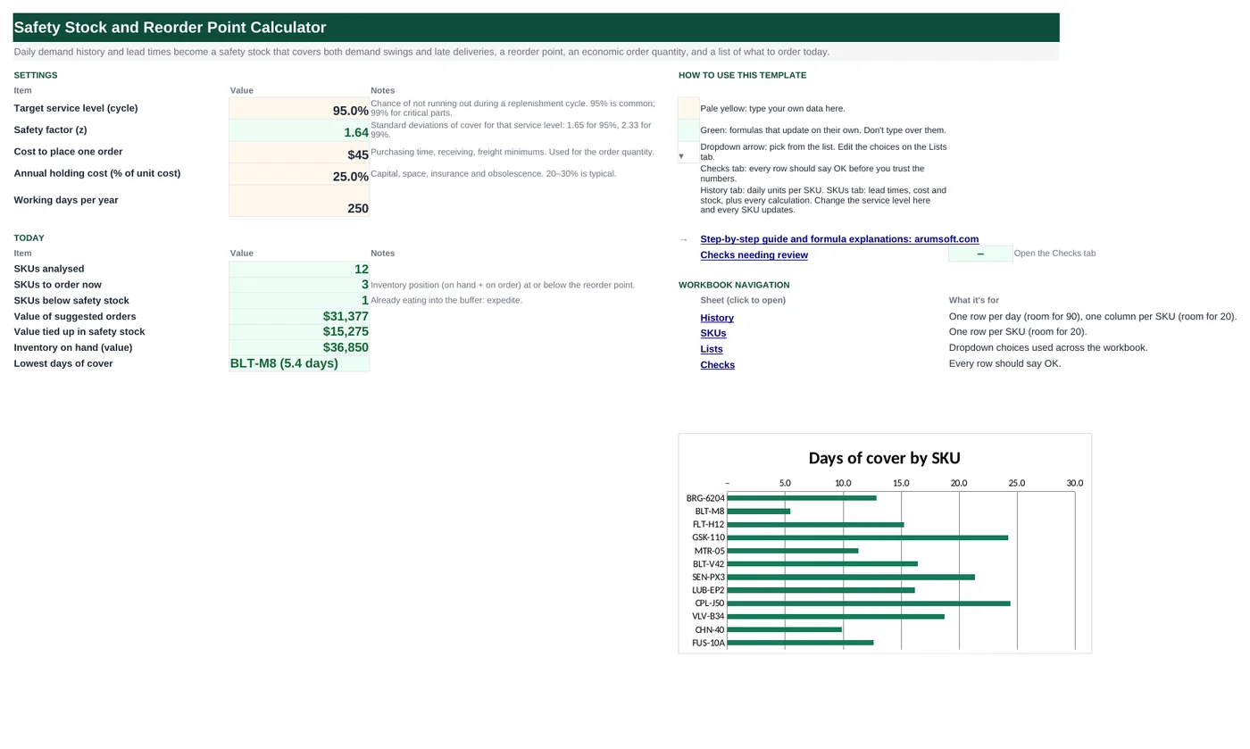
Reorder too late and you stock out; carry too much and cash sits on a shelf. This workbook reads 90 days of daily demand for each SKU, measures how much demand and supplier lead time swing, and turns your chosen service level into a safety stock, a reorder point and an economic order quantity. It then compares stock on hand and on order with the reorder point and tells you what to order today.
- Sheets:
- 5
- Works with:
- Excel for Microsoft 365, Excel 2016 or later, Excel for Mac and Excel for the web
- Updated:
What you can do with it
- Average and standard deviation of daily demand per SKU, read straight from a 90-day history
- Safety stock that covers both demand and lead-time variability at your service level (z from NORM.S.INV)
- Reorder point, EOQ, days of cover and status: OK, Order now or Below safety stock
- Suggested order quantity, value of orders and of safety stock, with a days-of-cover chart
What's inside
The workbook has 5 sheets. You only type on a few of them; the rest calculate.
| Sheet | What it's for | You enter | Calculated for you |
|---|---|---|---|
| Start Here | Settings and the order summary | Service level, cost per order, holding cost %, working days per year | z-score, SKUs analysed, SKUs to order now, below safety stock, value of suggested orders, safety stock value, stock on hand, lowest days of cover |
| History | 90 days × 20 SKUs of daily demand | Date, one column of units per SKU | Nothing |
| SKUs | One row per SKU (20) | SKU, description, lead time and its variation, unit cost, optional service-level override, on hand, on order | Demand mean and spread, z, lead-time demand, safety stock, reorder point, annual demand, EOQ, days of cover, status, suggested order |
| Lists | Service levels | Common service levels | Nothing |
| Checks | Six data checks | Nothing | OK or Review |
Before you start
- Export daily sales or usage per SKU for the last 90 days (zero on days with no demand, not blank).
- Measure lead time from your purchase orders: average days from order to receipt, and how many days it typically varies.
- Decide which items deserve a higher service level: anything that stops production or loses a customer.
Step-by-step guide
Set the service level and costs
Start Here B6–B10: service level (95% means a stockout in about one replenishment cycle in twenty), cost to place an order, yearly holding cost as a % of item value, and working days per year.
Paste demand history
History tab: dates down column A, SKU codes across row 4, daily units underneath. The SKUs tab finds each SKU's column by its code.
Describe each SKU
SKUs tab: SKU code (matching the History header), description, average lead time and its standard deviation in days, unit cost and, if needed, a higher service level in column I.
Enter stock positions
Column Q on hand and column R already on order.
Read the status
Column T: Below safety stock (expedite), Order now (at or under the reorder point) or OK. Column U gives the quantity to order.
Order and repeat
Place the orders, add the quantities to On order, and refresh the history each week or month.
Formula map
Every formula in the workbook, grouped by the sheet and column it lives in. A column of copied formulas counts once; the range it covers is shown.
| Sheet | Cells | Functions | What it computes | Reads | Feeds |
|---|---|---|---|---|---|
| Start Here | B7 | NORM.S.INV | z-score for the service level | B6 | Used for every SKU without an override. |
| SKUs | D5 copied down to row 24 | IF, IFERROR, AVERAGE, INDEX, MATCH | Average daily demand | A5 | Lead-time demand, annual demand and days of cover all use it. |
| SKUs | E5 copied down to row 24 | IF, IFERROR, STDEV, INDEX, MATCH | Demand variability | D5 | The demand part of the safety-stock formula. |
| SKUs | M5 copied down to row 24 | IF, ROUNDUP, SQRT | Safety stock | K5, F5, E5, D5, G5 | Part of the reorder point; stock below it means expedite. |
| SKUs | N5 copied down to row 24 | IF, ROUNDUP | Reorder point | L5, M5 | The trigger for the status column. |
| SKUs | P5 copied down to row 24 | IF, OR, ROUNDUP, SQRT | Economic order quantity | O5, H5 | The minimum suggested order. |
| SKUs | T5 copied down to row 24 | IF | Stock status | Q5, R5, M5, N5 | Colored and counted on Start Here. |
| SKUs | U5 copied down to row 24 | IF, OR, MAX | Suggested order | T5, P5, N5, M5, Q5, R5 | Summed in value on Start Here B17. |
| Start Here | B17 | SUMPRODUCT, IFERROR | Value of suggested orders | — | The cash you need for this round of purchasing. |
Every formula, explained
Each formula below is copied straight from the file, so what you read here is exactly what the cell contains. Click any cell in Excel to see it in the formula bar.
=NORM.S.INV(B6)Turns a service level into the number of standard deviations of buffer it needs, using the inverse of the standard normal distribution.
Piece by piece
NORM.S.INV(B6)- 95% → 1.645; 99% → 2.326; 90% → 1.282.
With the sample data: B6 = 95.0% → B7 result 1.64
How it is used: Used for every SKU without an override.
How to change it: Change B6; z follows.
Learn this: Essential Excel Functions: SUM, AVERAGE, COUNT, MIN and MAX →=IF(A5="", "", IFERROR(AVERAGE(INDEX(History!$B$5:$U$94, 0, MATCH(A5, History!$B$4:$U$4, 0))),
0))Finds this SKU's column in the History sheet by its code and averages it.
Piece by piece
MATCH(A5, History!$B$4:$U$4, 0)- Which column holds this SKU.
INDEX(History!$B$5:$U$94, 0, …)- Row 0 returns the whole column.
AVERAGE(…)- Mean units per day.
IFERROR(…, 0)- Zero if the code is not in the history.
With the sample data: A5 = BRG-6204 → D5 result 40.36
How it is used: Lead-time demand, annual demand and days of cover all use it.
How to change it: Nothing to change.
Learn this: How to Use INDEX and MATCH in Excel →=IF(A5="", "", IFERROR(STDEV(INDEX(History!$B$5:$U$94, 0, MATCH(A5, History!$B$4:$U$4, 0))),
0))Standard deviation of the same column: how much a typical day differs from the average.
Piece by piece
STDEV(INDEX(…, 0, MATCH(…)))- Sample standard deviation of daily demand.
With the sample data: D5 = 40.36 → E5 result 13.57
How it is used: The demand part of the safety-stock formula.
How to change it: Nothing to change.
Learn this: How to Use INDEX and MATCH in Excel →=IF(A5="", "", ROUNDUP(K5*SQRT(F5*E5^2+D5^2*G5^2), 0))The buffer that covers both demand swings during the lead time and late deliveries: z times the combined standard deviation, rounded up to whole units.
Piece by piece
F5*E5^2- Demand variance over the average lead time.
D5^2*G5^2- Extra demand while a late order is awaited.
SQRT(…)- Combined standard deviation of lead-time demand.
K5*…- Times z for the service level.
ROUNDUP(…, 0)- Whole units, never short.
With the sample data: K5 = 1.64, F5 = 7, E5 = 13.57, D5 = 40.36, G5 = 1.5 → M5 result 116
How it is used: Part of the reorder point; stock below it means expedite.
How to change it: If lead time never varies, set G5 to 0 and the formula reduces to z × σ × √LT.
Learn this: How to Round Numbers in Excel: ROUND, ROUNDUP and ROUNDDOWN →=IF(A5="", "", ROUNDUP(L5+M5, 0))Expected demand during the lead time plus safety stock. When stock on hand plus on order falls to this level, order.
Piece by piece
L5- Average daily demand × average lead time.
+M5- Safety stock.
With the sample data: L5 = 282.49, M5 = 116 → N5 result 399
How it is used: The trigger for the status column.
How to change it: Nothing to change.
Learn this: How to Round Numbers in Excel: ROUND, ROUNDUP and ROUNDDOWN →=IF(OR(A5="", H5=0), "", ROUNDUP(SQRT(2*O5*'Start Here'!$B$8/(H5*'Start Here'!$B$9)),
0))The order size that balances ordering cost against holding cost: the square root of 2 × annual demand × cost per order ÷ yearly holding cost per unit.
Piece by piece
O5- Annual demand (daily × working days).
'Start Here'!$B$8- Cost per order.
H5*'Start Here'!$B$9- Holding cost per unit per year.
SQRT(2*…/…)- The EOQ formula.
With the sample data: O5 = 10,088.89, H5 = 3.1 → P5 result 1,083
How it is used: The minimum suggested order.
How to change it: Round to your supplier's pack or pallet size after reading it.
Learn this: How to Round Numbers in Excel: ROUND, ROUNDUP and ROUNDDOWN →=IF(A5="", "", IF(Q5<M5, "Below safety stock",
IF(Q5+R5<=N5, "Order now", "OK")))Below safety stock if on-hand alone is under the buffer; Order now if on hand plus on order is at or under the reorder point; otherwise OK.
Piece by piece
Q5<M5- Already eating the buffer.
Q5+R5<=N5- Inventory position at the trigger.
With the sample data: Q5 = 520, R5 = 0, M5 = 116, N5 = 399 → T5 result OK
How it is used: Colored and counted on Start Here.
How to change it: Nothing to change.
Learn this: How to Use the IF Function in Excel →=IF(OR(A5="", T5="OK"), 0, MAX(P5, N5+M5-Q5-R5))Orders enough to bring the inventory position back above the reorder point plus a safety-stock margin, but never less than the EOQ.
Piece by piece
T5="OK"- No order: 0.
N5+M5-Q5-R5- Gap to the reorder point plus a buffer.
MAX(P5, …)- At least one economic order.
With the sample data: T5 = OK, P5 = 1,083, N5 = 399, M5 = 116, Q5 = 520, R5 = 0 → U5 result 0
How it is used: Summed in value on Start Here B17.
How to change it: Replace with your own order-up-to rule if you use one.
Learn this: How to Use MIN and MAX in Excel →=SUMPRODUCT(IFERROR(SKUs!$U$5:$U$24*SKUs!$H$5:$H$24, 0))Multiplies each suggested quantity by its unit cost and adds them up.
Piece by piece
SKUs!$U$5:$U$24*SKUs!$H$5:$H$24- Quantity × cost per row.
IFERROR(…, 0)- Ignores empty rows.
SUMPRODUCT(…)- Adds the products.
With the sample data: B17 result 31,377
How it is used: The cash you need for this round of purchasing.
How to change it: Nothing to change.
Learn this: How to Use IFERROR in Excel →Tips and limits
- Capacity: 20 SKUs and 90 days of history. For more SKUs, insert rows inside the SKUs table and columns inside History B:U.
- Use at least 60–90 days of history; fewer days make the standard deviation unreliable. Remove one-off bulk orders that will not repeat.
- The formula assumes demand is roughly normal. For very slow movers (a few units a month) set a minimum by judgement instead.
- A 99% service level costs far more stock than 95%: compare the safety stock value on Start Here before raising it everywhere.
- Lead time variability is often the bigger driver. Measure it from receipts, not from what the supplier quotes.
Learn the skills behind this template
Was this guide helpful? Spot a mistake? Send feedback · admin@arumsoft.com