OEE Calculator for Excel (Overall Equipment Effectiveness)
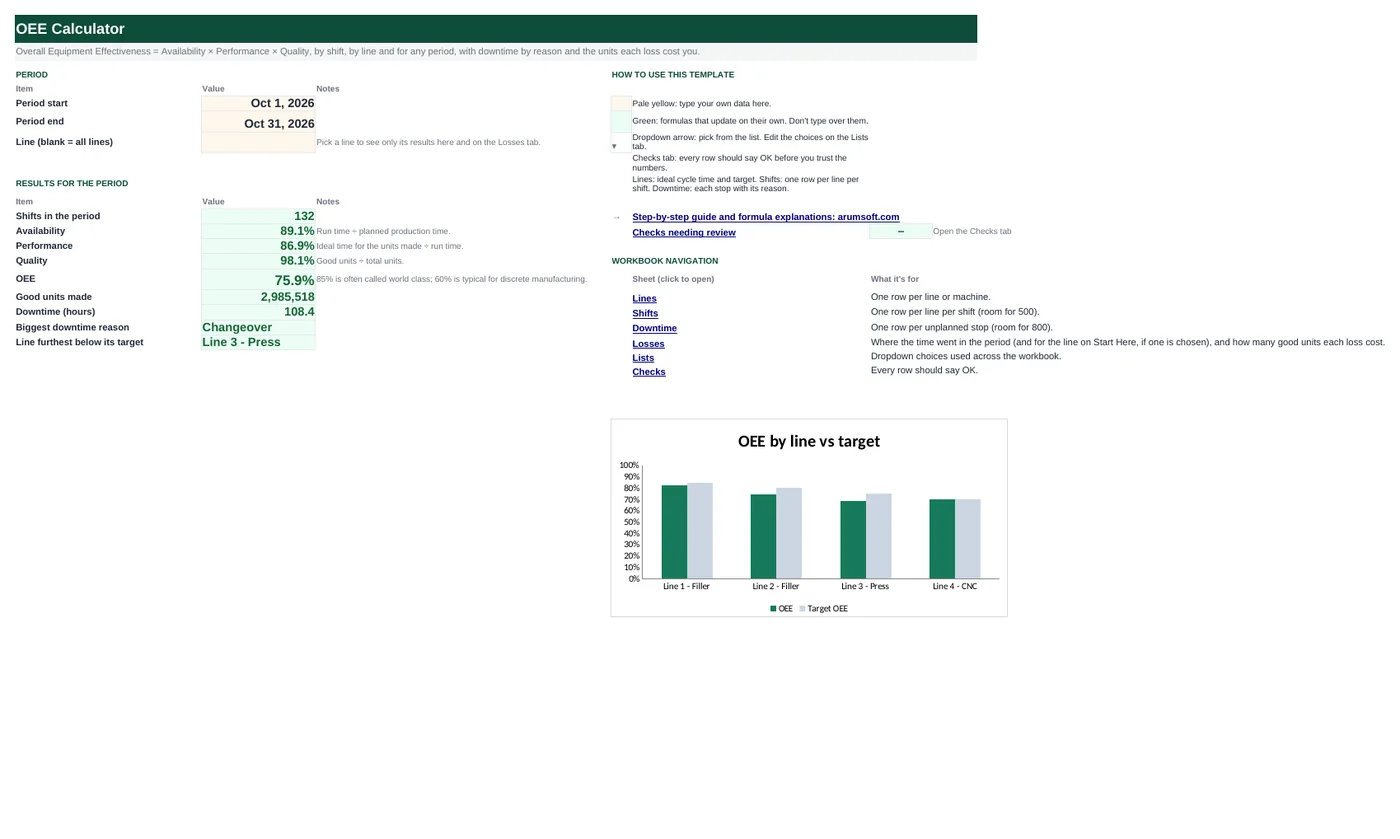
OEE answers one question: of the time a line was scheduled to run, how much produced good parts at full speed? It splits the answer into three losses you can act on: availability (stops), performance (running slower than the ideal cycle) and quality (rejects). This workbook takes a short log per shift and a downtime log, works out all three for every shift, rolls them up correctly by line and period, ranks downtime reasons, and turns each loss into units you did not make.
- Sheets:
- 7
- Works with:
- Excel for Microsoft 365, Excel 2016 or later, Excel for Mac and Excel for the web
- Updated:
What you can do with it
- Availability, performance, quality and OEE for every shift, with a heat-map
- Period and line totals rolled up from sums of minutes and units, not averages of percentages
- Downtime minutes, hours, share and stops by reason for any period or line
- Capacity at ideal speed split into availability, performance and quality losses in units
What's inside
The workbook has 7 sheets. You only type on a few of them; the rest calculate.
| Sheet | What it's for | You enter | Calculated for you |
|---|---|---|---|
| Start Here | Period, line filter and results | Period start and end, optional line | Shifts, availability, performance, quality, OEE, good units, downtime hours, top downtime reason, line furthest below target |
| Lines | One row per line (10) | Line, product, ideal cycle time, target OEE | Shifts, A, P, Q, OEE, good units and gap to target for the period |
| Shifts | One row per line per shift (500) | Date, line, shift, shift length, planned stops, total units, rejects | Planned production time, downtime, run time, ideal cycle, A, P, ideal run time, good units, Q, OEE |
| Downtime | One row per stop (800) | Date, line, shift, minutes, reason | Match to a logged shift |
| Losses | Where time and units went | Nothing | Downtime by reason; capacity split into losses and good units |
| Lists | Dropdowns | Shifts and downtime reasons | Nothing |
| Checks | Six data checks | Nothing | OK or Review |
Before you start
- Find the ideal cycle time for each line: the nameplate rate or the best sustained rate you have ever seen, in seconds per unit.
- Decide what counts as planned stops (breaks, meetings, planned maintenance). Everything else is downtime.
- Agree a short list of downtime reasons; the Losses tab is only as good as the reasons people pick.
Step-by-step guide
Describe the lines
Lines tab: name, product, ideal cycle time in seconds per unit, and the OEE target.
Log every shift
Shifts tab: date, line, shift, shift length and planned stops in minutes, total units made and rejects.
Log every stop
Downtime tab: the same date, line and shift, minutes stopped and a reason. They add up into the shift's downtime automatically.
Pick the period
Start Here B6 and B7; leave B8 blank for all lines or pick one.
Read the three losses
Start Here shows A, P, Q and OEE. Lines compares each line with its target.
Attack the biggest loss
Losses tab: the downtime reasons ranked, and how many good units each type of loss cost.
Formula map
Every formula in the workbook, grouped by the sheet and column it lives in. A column of copied formulas counts once; the range it covers is shown.
| Sheet | Cells | Functions | What it computes | Reads | Feeds |
|---|---|---|---|---|---|
| Shifts | I5 copied down to row 504 | IF, SUMIFS | Downtime for the shift | A5, B5, C5 | Run time = planned production time − downtime. |
| Shifts | L5 copied down to row 504 | IF, OR | Availability | J5, H5 | First of the three OEE factors. |
| Shifts | K5 copied down to row 504 | IF, IFERROR, INDEX, MATCH | Ideal cycle time for the line | B5 | Performance and the loss calculations use it. |
| Shifts | M5 copied down to row 504 | IF, OR | Performance | N5, J5 | Above 100% means the ideal cycle is set too slow; the check flags it. |
| Shifts | Q5 copied down to row 504 | IF, OR | OEE for the shift | L5, M5, P5 | Colored from red (40%) to green (85%). |
| Start Here | B13 | IFERROR, SUMIFS, IF | Availability for the period | — | B14 and B15 do the same for performance and quality; B16 multiplies them. Summing first, then dividing, weights long shifts properly. |
| Lines | I5 copied down to row 14 | IF | OEE by line | F5, G5, H5 | Compared with the target in column K and charted on Start Here. |
| Losses | B5 copied down to row 14 | IF, SUMIFS | Downtime minutes by reason | — | The largest reason is shown on Start Here. |
| Losses | B19 | SUMPRODUCT, IF, IFERROR | Units lost to downtime | — | Capacity minus availability, performance and quality losses equals good units. |
Every formula, explained
Each formula below is copied straight from the file, so what you read here is exactly what the cell contains. Click any cell in Excel to see it in the formula bar.
=IF(A5="", "", SUMIFS(Downtime!$D$5:$D$804,
    Downtime!$A$5:$A$804, A5,
    Downtime!$B$5:$B$804, B5,
    Downtime!$C$5:$C$804, C5))
Adds the minutes on the Downtime tab with the same date, line and shift.
Piece by piece
Downtime!$D$5:$D$804- Minutes to add.
Downtime!$A$5:$A$804, A5- Same date.
Downtime!$B$5:$B$804, B5- Same line.
Downtime!$C$5:$C$804, C5- Same shift.
With the sample data: A5 = Sep 1, 2026, B5 = Line 1 - Filler, C5 = Day → I5 result 62
How it is used: Run time = planned production time − downtime.
How to change it: Nothing to change.
Learn this: How to Use SUMIF and SUMIFS in Excel →=IF(OR(A5="", N(H5)=0), "", J5/H5)Run time divided by planned production time (shift length minus planned stops).
Piece by piece
J5- Run time in minutes.
/H5- Planned production time.
With the sample data: J5 = 388, H5 = 450 → L5 result 86.2%
How it is used: First of the three OEE factors.
How to change it: Nothing to change.
Learn this: How to Write Basic Formulas in Excel →=IF(A5="", "", IFERROR(INDEX(Lines!$C$5:$C$14, MATCH(B5, Lines!$A$5:$A$14, 0)),
""))Looks up the line's ideal seconds per unit on the Lines tab.
Piece by piece
MATCH(B5, Lines!$A$5:$A$14, 0)- Row of the line.
INDEX(Lines!$C$5:$C$14, …)- Its ideal cycle.
With the sample data: B5 = Line 1 - Filler → K5 result 50.0%
How it is used: Performance and the loss calculations use it.
How to change it: Change it on the Lines tab.
Learn this: How to Use INDEX and MATCH in Excel →=IF(OR(A5="", N(J5)=0, N5=""), "", N5/J5)How long the units made should have taken at ideal speed, divided by the time the line actually ran.
Piece by piece
N5 = K5*F5/60- Ideal run time in minutes: seconds per unit × units ÷ 60.
/J5- Run time.
With the sample data: N5 = 362.7, J5 = 388 → M5 result 93.5%
How it is used: Above 100% means the ideal cycle is set too slow; the check flags it.
How to change it: Nothing to change.
Learn this: How to Write Basic Formulas in Excel →=IF(OR(L5="", M5="", P5=""), "", L5*M5*P5)Availability × performance × quality.
Piece by piece
L5- Availability.
*M5- Performance.
*P5- Quality = good ÷ total units.
With the sample data: L5 = 86.2%, M5 = 93.5%, P5 = 98.6% → Q5 result 79.5%
How it is used: Colored from red (40%) to green (85%).
How to change it: Nothing to change.
Learn this: How to Write Basic Formulas in Excel →=IFERROR(SUMIFS(Shifts!$J$5:$J$504,
Shifts!$A$5:$A$504, ">="&B6,
Shifts!$A$5:$A$504, "<="&B7,
Shifts!$B$5:$B$504, IF(B8="", "*", B8))/SUMIFS(Shifts!$H$5:$H$504,
Shifts!$A$5:$A$504, ">="&B6,
Shifts!$A$5:$A$504, "<="&B7,
Shifts!$B$5:$B$504, IF(B8="", "*", B8)),
0)Total run time ÷ total planned production time for shifts in the period, for one line or all of them.
Piece by piece
Shifts!$J$5:$J$504- Run time to add.
Shifts!$A$5:$A$504, ">="&B6, …, "<="&B7- Dates in the period.
Shifts!$B$5:$B$504, IF(B8="", "*", B8)- The chosen line, or "*" (any text) for all lines.
/SUMIFS(Shifts!$H$5:$H$504, …)- Planned production time, same criteria.
With the sample data: B13 result 89.1%
How it is used: B14 and B15 do the same for performance and quality; B16 multiplies them. Summing first, then dividing, weights long shifts properly.
How to change it: Change the period and line in B6–B8.
Learn this: How to Use SUMIF and SUMIFS in Excel →=IF(N(E5)=0, "", F5*G5*H5)The line's availability, performance and quality for the period multiplied together.
Piece by piece
F5- Availability for the line.
*G5*H5- Performance × quality.
With the sample data: F5 = 91.8%, G5 = 91.4%, H5 = 98.5% → I5 result 82.6%
How it is used: Compared with the target in column K and charted on Start Here.
How to change it: Nothing to change.
Learn this: How to Write Basic Formulas in Excel →=IF(A5="", "", SUMIFS(Downtime!$D$5:$D$804,
Downtime!$A$5:$A$804, ">="&'Start Here'!$B$6,
Downtime!$A$5:$A$804, "<="&'Start Here'!$B$7,
Downtime!$B$5:$B$804, IF('Start Here'!$B$8="", "*", 'Start Here'!$B$8),
Downtime!$E$5:$E$804, A5))Adds downtime for this reason within the period (and line, if one is chosen).
Piece by piece
Downtime!$D$5:$D$804- Minutes.
Downtime!$A$5:$A$804, ">="&'Start Here'!$B$6, …- Period.
Downtime!$B$5:$B$804, IF('Start Here'!$B$8="", "*", …)- Line filter.
Downtime!$E$5:$E$804, A5- Reason.
With the sample data: B5 result 1,738
How it is used: The largest reason is shown on Start Here.
How to change it: Edit the reason list on the Lists tab.
Learn this: How to Use SUMIF and SUMIFS in Excel →=SUMPRODUCT((Shifts!$A$5:$A$504>='Start Here'!$B$6)*(Shifts!$A$5:$A$504<='Start Here'!$B$7)*IF('Start Here'!$B$8="",
1, Shifts!$B$5:$B$504='Start Here'!$B$8)*IFERROR(Shifts!$I$5:$I$504*60/Shifts!$K$5:$K$504,
0))For each shift, downtime minutes × 60 ÷ ideal seconds per unit: the units the line could have made while stopped.
Piece by piece
(Shifts!$A$5:$A$504>=…)*(…<=…)- Shifts in the period.
IF('Start Here'!$B$8="", 1, Shifts!$B$5:$B$504=…)- Line filter.
IFERROR(Shifts!$I$5:$I$504*60/Shifts!$K$5:$K$504, 0)- Lost units per shift.
SUMPRODUCT(…)- Added up.
With the sample data: B19 result 361,780.33
How it is used: Capacity minus availability, performance and quality losses equals good units.
How to change it: Nothing to change.
Learn this: How to Use IFERROR in Excel →Tips and limits
- Capacity: 10 lines, 500 shifts, 800 downtime entries. Start a new file each quarter or extend the ranges.
- Never average OEE percentages across shifts; sum the minutes and units first, as Start Here and Lines do.
- Use one ideal cycle per line. If a line runs several products at different speeds, add a line row per product, or log performance by product.
- Short stops under a minute or two are hard to log; they show up as performance loss instead, which is fine.
- 85% is a common world-class benchmark; most plants start between 40% and 65%. Compare a line with its own history first.
Learn the skills behind this template
Was this guide helpful? Spot a mistake? Send feedback · admin@arumsoft.com