HOA Budget and Reserve Planner for Excel
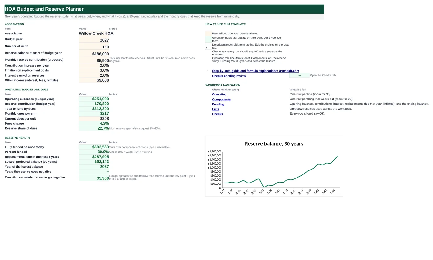
An HOA board has two numbers to get right: next year's operating budget and the reserve contribution that keeps roofs and pavement from becoming special assessments. This workbook builds the operating budget line by line, lists every reserve component with its last replacement, useful life and cost, computes the fully funded balance and percent funded, and runs a 30-year funding plan with inflated replacements, interest and rising contributions. The dues per unit fall out at the end, with a check that the reserve never goes negative.
- Sheets:
- 6
- Works with:
- Excel for Microsoft 365, Excel 2016 or later, Excel for Mac and Excel for the web
- Updated:
What you can do with it
- Operating budget vs prior year with per-unit-per-month cost
- Reserve components: next replacement year, remaining life, inflated cost, fully funded balance, annual accrual
- 30-year funding plan with repeat replacements, inflation, interest and contribution increases
- Monthly dues per unit, reserve share of dues, percent funded and the contribution needed to stay solvent
What's inside
The workbook has 6 sheets. You only type on a few of them; the rest calculate.
| Sheet | What it's for | You enter | Calculated for you |
|---|---|---|---|
| Start Here | Association settings, dues and reserve health | Units, reserve balance, monthly contribution, increase %, inflation, interest, other income, current dues | Operating total, reserve contribution, total to fund, dues per unit and change, reserve share, fully funded balance, % funded, 5-year replacements, lowest balance and year, years negative, contribution needed |
| Operating | Line items (30) | Line, prior-year actual, budget | Change, change %, per unit per month, totals |
| Components | Reserve components (30) | Component, last replaced, useful life, current cost | Next replacement, remaining life, age, inflated cost, fully funded balance, annual accrual |
| Funding | 30 years | Nothing | Opening, contributions, interest, replacements, net change, ending, status |
| Lists | Reference | Notes | Nothing |
| Checks | Six checks | Nothing | OK or Review |
Before you start
- Get last year's actuals by line from the management company or the bank statements.
- List every common element that wears out, with the year it was last replaced, how long it lasts and what it costs today; a reserve study, if you have one, has this list.
- Know the current reserve balance and the dues per unit today.
Step-by-step guide
Set the association
Start Here B6–B14: units, reserve balance, proposed monthly contribution, annual increase, inflation, interest and other income.
Build the operating budget
Operating tab: prior-year actual and budget per line. Lines up more than 10% are highlighted; per-unit-per-month shows what each line costs an owner.
List the reserve components
Components tab: last replaced, useful life, current cost. Next replacement, inflated cost, fully funded balance and annual accrual calculate; items due within 3 years are highlighted.
Read reserve health
Start Here B28–B30: fully funded balance, percent funded (under 30% is weak), and replacements due in the next five years.
Check the 30-year plan
Funding tab and Start Here B31–B34: the lowest projected balance and its year, how many years go negative, and a rough contribution that keeps the balance above zero. Adjust B10 until it does.
Set the dues
Start Here B18–B24: operating plus reserve less other income, divided by units and twelve, compared with current dues, and the reserve share of dues.
Formula map
Every formula in the workbook, grouped by the sheet and column it lives in. A column of copied formulas counts once; the range it covers is shown.
| Sheet | Cells | Functions | What it computes | Reads | Feeds |
|---|---|---|---|---|---|
| Components | D5 copied down to row 34 | IF, MAX | Next replacement year | B5, C5 | The Funding tab looks for this year and its repeats. |
| Components | H5 copied down to row 34 | IF | Inflated cost at replacement | F5, E5 | What the Funding tab charges in the replacement year. |
| Components | I5 copied down to row 34 | IF, OR | Fully funded balance | F5, G5, C5 | Summed on Start Here B28; percent funded = actual ÷ this. |
| Funding | C5 copied down to row 34 | arithmetic | Contributions in a year | A5 | Added to the opening balance. |
| Funding | E5 copied down to row 34 | SUMIF, SUMPRODUCT, IFERROR, MOD | Replacements in a year | A5 | The big outflows in the 30-year chart. |
| Funding | G5 copied down to row 34 | arithmetic | Ending balance | B5, F5 | Next year's opening; the minimum is the solvency test. |
| Funding | H5 copied down to row 33 | IF | Status | G5, E6 | Colored by conditional formatting. |
| Start Here | B21 | IF, ROUND | Monthly dues per unit | B20, B8 | Compared with current dues in B23. |
| Start Here | B29 | IF | Percent funded | B9, B28 | The standard reserve-study health measure. |
| Start Here | B34 | IF, ROUND, MIN, MATCH | Contribution needed to never go negative | B33, B10, B31 | Type it into B10 and re-check; interest and increases make it slightly conservative. |
Every formula, explained
Each formula below is copied straight from the file, so what you read here is exactly what the cell contains. Click any cell in Excel to see it in the formula bar.
=IF(A5="", "", MAX(B5+C5, 'Start Here'!$B$7))Last replaced plus useful life, but never earlier than the budget year so an overdue item lands in year one.
Piece by piece
B5+C5- Last replaced + useful life.
'Start Here'!$B$7- The budget year.
MAX(…, …)- Whichever is later.
With the sample data: B5 = 2,021, C5 = 5 → D5 result 2,027
How it is used: The Funding tab looks for this year and its repeats.
How to change it: Nothing to change.
Learn this: How to Use MIN and MAX in Excel →=IF(A5="", "", F5*(1+'Start Here'!$B$12)^E5)Today's cost grown by inflation for the years until replacement.
Piece by piece
F5- Current cost.
(1+'Start Here'!$B$12)^E5- Inflation compounded over the remaining life.
With the sample data: F5 = 18,000, E5 = 0 → H5 result 18,000
How it is used: What the Funding tab charges in the replacement year.
How to change it: Nothing to change.
Learn this: How to Write Basic Formulas in Excel →=IF(OR(A5="", C5=0), "", F5*G5/C5)The share of the component's cost that should already be saved: cost × age ÷ useful life.
Piece by piece
F5- Current cost.
*G5- Age in years (capped at the useful life).
/C5- Divided by useful life.
With the sample data: F5 = 18,000, G5 = 5, C5 = 5 → I5 result 18,000
How it is used: Summed on Start Here B28; percent funded = actual ÷ this.
How to change it: Nothing to change.
Learn this: How to Write Basic Formulas in Excel →='Start Here'!$B$10*12*(1+'Start Here'!$B$11)^(A5-'Start Here'!$B$7)Monthly contribution × 12, increased by the annual rate for each year after the budget year.
Piece by piece
'Start Here'!$B$10*12- First-year contribution.
(1+'Start Here'!$B$11)^(A5-'Start Here'!$B$7)- Compounded increase.
With the sample data: A5 = 2,027 → C5 result 70,800
How it is used: Added to the opening balance.
How to change it: Nothing to change.
Learn this: How to Write Basic Formulas in Excel →=SUMIF(Components!$D$5:$D$34,
A5, Components!$H$5:$H$34)+SUMPRODUCT(IFERROR((Components!$D$5:$D$34<A5)*(MOD(A5-Components!$D$5:$D$34, Components!$C$5:$C$34)=0)*Components!$F$5:$F$34*(1+'Start Here'!$B$12)^(A5-'Start Here'!$B$7),
0))First replacements scheduled for this year (SUMIF on the Components tab) plus repeat replacements: components whose first replacement is earlier and where the years since divide evenly by the useful life, each inflated to this year.
Piece by piece
SUMIF(Components!$D$5:$D$34, A5, Components!$H$5:$H$34)- First replacements due this year.
(Components!$D$5:$D$34<A5)- Already replaced once.
MOD(A5-Components!$D$5:$D$34, Components!$C$5:$C$34)=0- A repeat falls in this year.
Components!$F$5:$F$34*(1+'Start Here'!$B$12)^(A5-'Start Here'!$B$7)- Cost inflated to this year.
SUMPRODUCT(IFERROR(…, 0))- Add them all, ignoring blank rows.
With the sample data: A5 = 2,027 → E5 result 18,000
How it is used: The big outflows in the 30-year chart.
How to change it: Nothing to change.
Learn this: How to Use SUMIF and SUMIFS in Excel →=B5+F5Opening plus contributions and interest minus replacements.
Piece by piece
B5- Opening balance.
+F5- Net change: contributions + interest − replacements.
With the sample data: B5 = 186,000, F5 = 56,520 → G5 result 242,520
How it is used: Next year's opening; the minimum is the solvency test.
How to change it: Nothing to change.
Learn this: How to Write Basic Formulas in Excel →=IF(G5<0, "Shortfall", IF(G5<E6*0.5, "Thin", "OK"))Shortfall when the ending balance is negative; Thin when it is under half of next year's replacements; OK otherwise.
Piece by piece
G5<0- Negative: Shortfall.
G5<E6*0.5- Less than half of next year's outflow: Thin.
With the sample data: G5 = 242,520, E6 = 74,160 → H5 result OK
How it is used: Colored by conditional formatting.
How to change it: Change 0.5 to your own comfort level.
Learn this: How to Use the IF Function in Excel →=IF(B8=0, 0, ROUND(B20/B8/12, 0))Operating expenses plus reserve contribution minus other income, divided by units and twelve, rounded to the dollar.
Piece by piece
B20- Total to fund by dues.
/B8- Per unit.
/12- Per month.
ROUND(…, 0)- Whole dollars.
With the sample data: B20 = 312,200, B8 = 120 → B21 result 217
How it is used: Compared with current dues in B23.
How to change it: Nothing to change.
Learn this: How to Round Numbers in Excel: ROUND, ROUNDUP and ROUNDDOWN →=IF(B28=0, 0, B9/B28)Actual reserve balance divided by the fully funded balance.
Piece by piece
B9- Reserve balance today.
/B28- Fully funded balance.
With the sample data: B9 = 186,000, B28 = 602,563.33 → B29 result 30.9%
How it is used: The standard reserve-study health measure.
How to change it: Nothing to change.
Learn this: How to Write Basic Formulas in Excel →=IF(B33=0, B10, ROUND(B10-MIN(Funding!$G$5:$G$34)/(12*MATCH(B31, Funding!$G$5:$G$34, 0)),
-2))If any year goes negative, spreads the worst shortfall over the months until that year and adds it to the current contribution; a rough starting point, rounded to $100.
Piece by piece
B33=0- No shortfall: keep the current contribution.
MIN(Funding!$G$5:$G$34)- The worst (most negative) balance.
MATCH(B31, Funding!$G$5:$G$34, 0)- Years until it happens.
B10-shortfall/(12*years)- Extra per month.
ROUND(…, -2)- To the nearest $100.
With the sample data: B33 = 0, B10 = 5,900, B31 = 52,142.16 → B34 result 5,900
How it is used: Type it into B10 and re-check; interest and increases make it slightly conservative.
How to change it: Nothing to change.
Learn this: How to Use INDEX and MATCH in Excel →Tips and limits
- Capacity: 30 operating lines, 30 components, 30 years. Extend components with Ctrl+H ($34).
- The 30-year plan is only as good as the component list. Walk the property with a contractor every three years and update lives and costs.
- Percent funded under 30% is the level at which lenders and buyers get nervous; some states require disclosure of it.
- A contribution increase of 3% a year with 3% inflation keeps pace; set the increase to 0% to see how fast a flat contribution falls behind.
- Keep the reserve in its own account. Mixing it with operating cash is how boards accidentally spend the roof.
Learn the skills behind this template
Was this guide helpful? Spot a mistake? Send feedback · admin@arumsoft.com