CRE Cap Rate and Sensitivity Analyzer for Excel
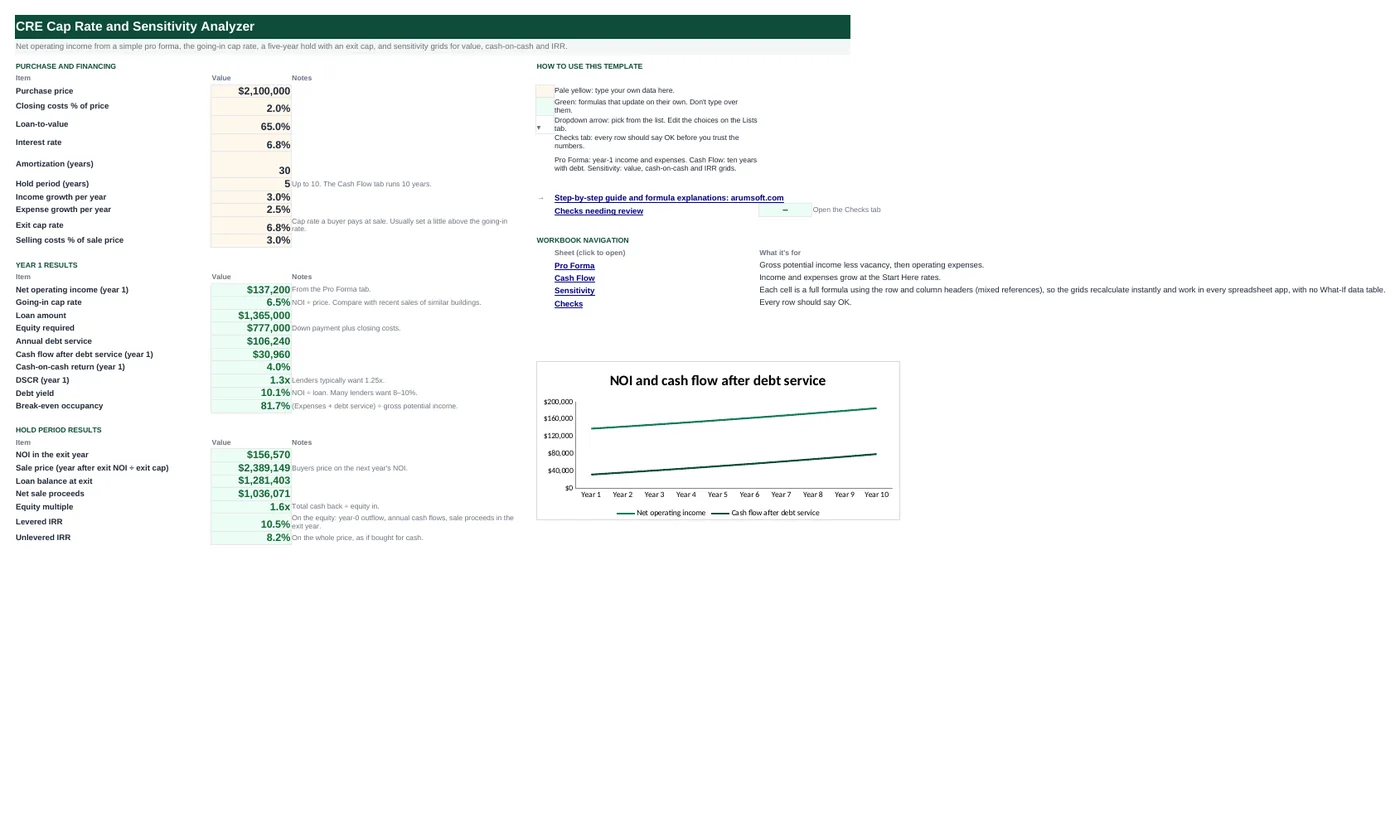
Underwriting a commercial property comes down to NOI, the cap rate you pay, the debt you put on it and the cap rate you sell at. This workbook builds NOI from a simple pro forma, prices the deal and the loan, runs ten years of cash flow with the loan amortizing, sells at the exit cap and returns equity multiple and IRR. Three sensitivity grids show value, cash-on-cash and equity multiple across cap rates, rates, leverage and growth, each cell a plain formula you can read.
- Sheets:
- 5
- Works with:
- Excel for Microsoft 365, Excel 2016 or later, Excel for Mac and Excel for the web
- Updated:
What you can do with it
- Year-1 NOI, going-in cap rate, DSCR, debt yield and break-even occupancy
- Ten-year cash flow with income and expense growth and an amortizing loan (CUMPRINC)
- Sale at the exit cap, net proceeds, equity multiple, levered and unlevered IRR
- Sensitivity grids for value (NOI × cap), cash-on-cash (rate × LTV) and equity multiple (exit cap × growth), no What-If data tables
What's inside
The workbook has 5 sheets. You only type on a few of them; the rest calculate.
| Sheet | What it's for | You enter | Calculated for you |
|---|---|---|---|
| Start Here | Inputs, year-1 results, hold-period results | Price, closing %, LTV, rate, amortization, hold, growth rates, exit cap, selling costs | NOI, cap rate, loan, equity, debt service, cash flow, cash-on-cash, DSCR, debt yield, break-even occupancy, exit NOI, sale price, loan balance, proceeds, equity multiple, IRRs |
| Pro Forma | Year-1 income and expenses | Income lines, vacancy %, expense lines | GPI, EGI, management fee, total expenses, NOI, expense ratio, NOI per unit |
| Cash Flow | Ten years | Nothing | EGI, expenses, NOI, debt service, cash flow, cash-on-cash, loan balance, DSCR, IRR streams |
| Sensitivity | Three 5×5 grids | Nothing (edit header offsets) | Value, cash-on-cash, equity multiple |
| Checks | Six underwriting checks | Nothing | OK or Review |
Before you start
- Get the trailing-12 income and expenses from the seller, and underwrite your own numbers for taxes (reassessed at sale), insurance and management.
- Know the lender's terms: LTV, rate, amortization, and the DSCR and debt yield they require.
- Pick an exit cap rate at or above today's, since you cannot know where rates will be in five years.
Step-by-step guide
Build the pro forma
Pro Forma tab: income lines, vacancy and credit loss %, expense lines. Management is 5% of EGI by formula. NOI and the expense ratio calculate.
Enter the deal
Start Here B6–B15: price, closing %, LTV, rate, amortization, hold period, income and expense growth, exit cap, selling costs.
Read year 1
Going-in cap rate, annual debt service, cash flow after debt service, cash-on-cash, DSCR, debt yield and break-even occupancy (B19–B28).
Read the hold
Exit-year NOI, the sale price (next year's NOI ÷ exit cap), loan balance at exit, net proceeds, equity multiple, levered and unlevered IRR (B32–B38).
Stress the deal
Sensitivity tab: value by NOI change × cap rate, cash-on-cash by rate × LTV, equity multiple by exit cap × income growth. The middle cell of each grid is the Start Here case.
Check the Checks
Cap rate in range, exit cap not below going-in, DSCR ≥ 1.25, hold between 1 and 10 years, expense ratio in range, and the grid centers matching Start Here.
Formula map
Every formula in the workbook, grouped by the sheet and column it lives in. A column of copied formulas counts once; the range it covers is shown.
| Sheet | Cells | Functions | What it computes | Reads | Feeds |
|---|---|---|---|---|---|
| Pro Forma | B22 | arithmetic | Net operating income | B11, B21 | Everything on Start Here starts from it. |
| Start Here | B20 | IF | Going-in cap rate | B19, B6 | The header of the value grid is built around it. |
| Start Here | B23 | IF, PMT | Annual debt service | B9, B10, B21 | Cash flow, DSCR and break-even occupancy use it. |
| Start Here | B28 | IF | Break-even occupancy | B23 | How much vacancy the deal can absorb before you feed it. |
| Cash Flow | F13 | IF, CUMPRINC | Loan balance at the end of year 5 | — | Start Here B34 picks the exit year's balance with INDEX. |
| Cash Flow | F15 | IF | Levered cash flow for IRR | F11 | Column A holds the year-0 equity outflow; Start Here B37 runs IRR over hold + 1 cells. |
| Start Here | B33 | IF, INDEX | Sale price | B11, B12, B14 | Net proceeds subtract selling costs and the loan balance. |
| Start Here | B37 | IFERROR, IRR, OFFSET | Levered IRR | B11 | The return on your equity including leverage. |
| Sensitivity | C7 copied down to row 10 | IF | Value at an NOI change and cap rate | — | The middle cell equals the purchase price when the going-in cap is used. |
| Sensitivity | C16 copied down to row 19 | PMT | Cash-on-cash at a rate and LTV | — | Shows how leverage cuts both ways as rates move. |
Every formula, explained
Each formula below is copied straight from the file, so what you read here is exactly what the cell contains. Click any cell in Excel to see it in the formula bar.
=B11-B21Effective gross income minus total operating expenses. No debt, no depreciation, no capex beyond reserves.
Piece by piece
B11- EGI = gross potential income × (1 − vacancy).
-B21- Total operating expenses.
With the sample data: B11 = 236,316, B21 = 99,115.8 → B22 result 137,200.2
How it is used: Everything on Start Here starts from it.
How to change it: Nothing to change.
Learn this: How to Write Basic Formulas in Excel →=IF(B6=0, 0, B19/B6)Year-1 NOI divided by the purchase price.
Piece by piece
B6=0- No price: 0.
B19/B6- NOI ÷ price.
With the sample data: B19 = 137,200.2, B6 = 2,100,000 → B20 result 6.5%
How it is used: The header of the value grid is built around it.
How to change it: Nothing to change.
Learn this: How to Write Basic Formulas in Excel →=IF(B21=0, 0, -PMT(B9/12, B10*12, B21)*12)Twelve monthly payments on the loan. PMT gives a negative payment, so it is negated.
Piece by piece
B9/12- Monthly rate.
B10*12- Number of payments.
B21- Loan amount.
-PMT(…)*12- Annual total, positive.
With the sample data: B9 = 6.8%, B10 = 30, B21 = 1,365,000 → B23 result 106,240.37
How it is used: Cash flow, DSCR and break-even occupancy use it.
How to change it: For interest-only, use B21*B9.
Learn this: Essential Excel Functions: SUM, AVERAGE, COUNT, MIN and MAX →=IF('Pro Forma'!$B$9=0, 0,
('Pro Forma'!$B$21+B23)/'Pro Forma'!$B$9)The occupancy at which NOI exactly covers debt service: (expenses + debt service) ÷ gross potential income.
Piece by piece
'Pro Forma'!$B$21- Operating expenses.
+B23- Debt service.
/'Pro Forma'!$B$9- Divided by gross potential income.
With the sample data: B23 = 106,240.37 → B28 result 81.7%
How it is used: How much vacancy the deal can absorb before you feed it.
How to change it: Nothing to change.
Learn this: How to Write Basic Formulas in Excel →=IF('Start Here'!$B$21=0,
0, 'Start Here'!$B$21+CUMPRINC('Start Here'!$B$9/12,
'Start Here'!$B$10*12, 'Start Here'!$B$21,
1, 5*12, 0))The original loan plus the cumulative principal paid through month 60 (CUMPRINC returns a negative number).
Piece by piece
'Start Here'!$B$9/12- Monthly rate.
'Start Here'!$B$10*12- Total periods.
'Start Here'!$B$21- Loan amount.
1, 60- From the first to the 60th payment.
0- Payments at period end.
With the sample data: F13 result 1,281,403.44
How it is used: Start Here B34 picks the exit year's balance with INDEX.
How to change it: Nothing to change.
Learn this: Essential Excel Functions: SUM, AVERAGE, COUNT, MIN and MAX →=F11+IF(5='Start Here'!$B$11, 'Start Here'!$B$35, 0)Cash flow after debt service, plus the net sale proceeds if this is the exit year.
Piece by piece
F11- Cash flow after debt service.
IF(5='Start Here'!$B$11, 'Start Here'!$B$35, 0)- Add sale proceeds in the exit year only.
With the sample data: F11 = 50,330.07 → F15 result 1,086,401.14
How it is used: Column A holds the year-0 equity outflow; Start Here B37 runs IRR over hold + 1 cells.
How to change it: Nothing to change.
Learn this: How to Use the IF Function in Excel →=IF(B14=0, 0, INDEX('Cash Flow'!$B$9:$K$9,
1, B11)*(1+B12)/B14)Buyers price on the NOI they will receive, so the exit-year NOI is grown one more year and divided by the exit cap.
Piece by piece
INDEX('Cash Flow'!$B$9:$K$9, 1, B11)- NOI in the exit year.
*(1+B12)- Grown one year.
/B14- Divided by the exit cap.
With the sample data: B11 = 5, B12 = 3.0%, B14 = 6.8% → B33 result 2,389,148.97
How it is used: Net proceeds subtract selling costs and the loan balance.
How to change it: To price on the exit-year NOI itself, remove *(1+B12).
Learn this: How to Use INDEX and MATCH in Excel →=IFERROR(IRR(OFFSET('Cash Flow'!$A$15, 0, 0, 1, B11+1)), "")IRR of the equity cash flows: year-0 equity out, annual cash flow after debt service, sale proceeds in the exit year. OFFSET takes exactly hold + 1 cells from the Cash Flow tab.
Piece by piece
OFFSET('Cash Flow'!$A$15, 0, 0, 1, B11+1)- Year 0 through the exit year.
IRR(…)- The rate that sets their present value to zero.
IFERROR(…, "")- Blank if IRR cannot converge.
With the sample data: B11 = 5 → B37 result 10.5%
How it is used: The return on your equity including leverage.
How to change it: Nothing to change.
Learn this: Essential Excel Functions: SUM, AVERAGE, COUNT, MIN and MAX →=IF(C$5=0, 0, 'Start Here'!$B$19*(1+$A7)/C$5)Year-1 NOI adjusted by the row's percentage, divided by the column's cap rate. $A7 locks the column, C$5 locks the row, so one formula fills the grid.
Piece by piece
'Start Here'!$B$19*(1+$A7)- NOI scaled by the row header.
/C$5- Divided by the column header cap rate.
With the sample data: C7 result 2,160,331.23
How it is used: The middle cell equals the purchase price when the going-in cap is used.
How to change it: Edit the header offsets to test other ranges.
Learn this: Relative, Absolute and Mixed References in Excel →=('Start Here'!$B$19+PMT($A16/12,
'Start Here'!$B$10*12, 'Start Here'!$B$6*C$14)*12)/('Start Here'!$B$6*(1-C$14)+'Start Here'!$B$6*'Start Here'!$B$7)Year-1 NOI minus the annual payment on a loan sized at the column's LTV and the row's rate, divided by the equity that LTV implies.
Piece by piece
PMT($A16/12, 'Start Here'!$B$10*12, 'Start Here'!$B$6*C$14)*12- Annual debt service at this rate and loan size (negative).
'Start Here'!$B$19+…- NOI minus debt service.
/('Start Here'!$B$6*(1-C$14)+'Start Here'!$B$6*'Start Here'!$B$7)- Equity: down payment plus closing costs.
With the sample data: C16 result 5.0%
How it is used: Shows how leverage cuts both ways as rates move.
How to change it: Nothing to change.
Learn this: Relative, Absolute and Mixed References in Excel →Tips and limits
- The exit cap is the biggest single assumption. The equity multiple grid shows the sample going from 1.6x at a 6.75% exit to 1.1x at 7.25% with 1% growth. Underwrite to the pessimistic corner, not the center.
- Taxes are usually reassessed at sale. Put the post-sale tax bill in the pro forma, not the seller's.
- Debt yield (NOI ÷ loan) is what lenders fall back on when cap rates move; 8–10% is a common floor.
- The grids use mixed references ($A7, C$5) so they work in Excel, Google Sheets, LibreOffice and Numbers. A What-If data table would not.
- For a value-add deal, model the stabilized NOI in year 2 or 3 by editing the Cash Flow growth rows directly; the IRR rows will follow.
Learn the skills behind this template
Was this guide helpful? Spot a mistake? Send feedback · admin@arumsoft.com